t-SNE

1. Introduction

t-SNE, or t-distributed stochastic neighbor embedding, is a dimensionality reduction technique. As opposed to classic techniques such as Principal Components Analysis (PCA) or classical multidimensional scaling (MDS), t-SNE provides non-linear and non-deterministic dimensionality reduction. Specifically, high-dimensional data is mapped to points in two or three-dimensions. According to van der Maaten et al., t-SNE is advantageous over many classic dimensionality reduction techniques in being able to capture the local structure of high-dimensional data well, while revealing global structure at several scales. Since t-SNE is non-deterministic, its main application is visualization of datasets [1].

2. Method

Let $\mathcal{X} = {x_1, x_2, \dots ,x_n}$ with $x_{i} \in \mathbb{R}^{d}$ denote the high dimensional dataset and let $\mathcal{Y} = {y_1, y_2, \dots ,y_n}$ denote the low-dimensional projections. t-SNE first defines a joint density $P(i, j) = p_{ij}$ that represents similarity between $x_{i}$ and $x_{j}$ and another joint density $Q(i, j) = q_{ij}$ that represents similarity between $y_{i}$ and $y_{j}$. t-SNE then finds projections $\mathcal{Y}$ to minimize the KL-divergence between $P$ and $Q$.

2.1 Similarity in high-dimensions

Define the similarity of $x_{j}$ to $x_i$ as the conditional probability $p_{j \lvert i}$ that $x_i$ would pick $x_j$ as its neighbor if neighbors were picked in proportion to their probability density under a Gaussian centered at $x_i$. This conditional probability $p_{j \lvert i}$ is given by

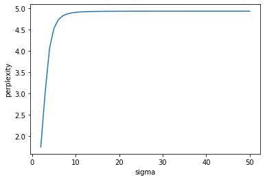
$$p_{j \lvert i} = \frac{\exp(-\lvert \lvert x_i - x_j\lvert \lvert^{2} / 2\sigma_{i}^{2})}{\sum_{k \neq i}\exp(-\lvert \lvert x_i - x_k \lvert \lvert^{2} / 2\sigma_{i}^{2})}$$

and $p_{i \lvert i} = 0$ for all $i$. Here $\sigma_i$ is the variance of the Gaussian centered and belonging to data point $x_i$. In t-SNE, the value of $\sigma_i$ for $x_i$ is chosen such that the perplexity equals a user-specified value, which is typically recommended to range from 5 - 50. Let $P_i$ denote the probability distribution of $x_i$, then perplexity is defined as

$$Perp(P_i) = 2^{H(P_i)},$$

where $H(P_i) = -\sum_{j}p_{j \lvert i}\log_{2}p_{j \lvert i}$ is the Shannon entropy of $P_i$. According to van der Maaten et al., the perplexity can be be interpreted as the effective number of neighbors. How is $\sigma_{i}$ chosen for each $x_i$? Since $Perp(P_i)$ increases monotonically with $\sigma_i$, the value of $\sigma_i$ is found via binary search.

%matplotlib inline
import random
import numpy as np
import matplotlib.pyplot as plt

def CreatePDist(distances, sigma):
    terms = [np.exp(-d / (2 * sigma**2)) for d in distances]
    normalization = sum(terms)
    return [num / normalization for num in terms]

def entropy(P):
    logTerms = [p * np.log(p) for p in P]
    return -sum(logTerms)

def perplexity(entropy):
    return 2**entropy

def randomDistances(minimum, maximum, n):
    return [random.randrange(minimum, maximum) for i in range(n)]

distances = randomDistances(0, 100, 10)
pSamples = [CreatePDist(distances, sigma) for sigma in range(2, 51, 1)]
entropies = [entropy(P) for P in pSamples]
perplexities = [perplexity(entropy) for entropy in entropies]
plt.plot(list(range(2, 51, 1)), perplexities);
plt.xlabel("sigma");
plt.ylabel("perplexity");

From $p_{j \lvert i}$, van der Maaten et al. constructed a joint probability distribution $p_{ij} = \frac{p_{j \lvert i} + p_{i \lvert j}}{2n}$ that represents similarity between $x_i$ and $x_j$. This ensures that $\sum_{j}p_{ij} = \frac{1 + \sum_{j}p_{i \lvert j}}{2n} > \frac{1}{2n}$, which means each datapoint $x_i$ is guaranteed a minimum contribution to the cost function that is a function of $p_{ij}$ that will be defined in greater detail later.

2.2 Similarity in low-dimensions

The similarity between two projected points $y_i$ and $y_j$ is defined as

$$q_{ij} = \frac{(1 + ||y_{i} - y_{j}||^{2})^{-1}}{\sum_{k \neq l}(1 + ||y_{k} - y_{l}||^{2})^{-1}},$$

involving a Student t-distribution with one degree of freedom, which is the same as a Cauchy distribution. As before, $q_{ii} = 0$ for all $i$. This distribution choice is because pairwise distances in a low-dimensional map cannot faithfully model distances between points in high-dimensions. Specifically, as the dimensionality $m$ increases, most of the points $x$ picked at random in a sphere will be close to the surface. To illustrate via simulation:

from numpy.linalg import norm

npoints = 1000
plt.figure(figsize=(15, 4))
for i, D in enumerate((2, 10, 20)):
    # Normally distributed points.
    u = np.random.randn(npoints, D)
    # Now on the sphere.
    u /= norm(u, axis=1)[:, None]
    # Uniform radius.
    r = np.random.rand(npoints, 1)
    # Uniformly within the ball.
    points = u * r**(1./D)
    # Plot.
    ax = plt.subplot(1, 3, i+1)
    ax.set_xlabel('Ball radius')
    if i == 0:
        ax.set_ylabel('Distance from origin')
    ax.hist(norm(points, axis=1),
            bins=np.linspace(0., 1., 50))
    ax.set_title('D=%d' % D, loc='left')

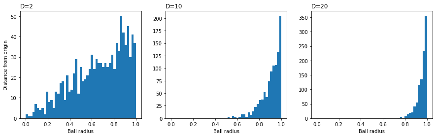
In a low-dimensional map, there is less space to accomodate the number of points at moderate distances from the center, leading to the crowding problem. The t-distribution has fatter tails than the Gaussian distribution, which means data points $x_{i}$ and $x_{j}$ need to be mapped to further separated map points $y_{i}$ and $y_{j}$ in order for $p_{ij}$ and $q_{ij}$ to be similar.

2.3 Cost function

The cost function is the KL-divergence between $P$ and $Q$

$$C = KL(P \lvert \lvert Q) = \sum_{i}\sum_{j}p_{ij}\log \frac{p_{ij}}{q_{ij}},$$

which is asymmetric $KL(P \lvert \lvert Q) \neq KL(Q \lvert \lvert P)$. The consequence for the fitted distribution $q$ for distribution $p$ as a result of this asymmetry is illustrated in the below diagram provided by Goodfellow [2].

Roughly speaking, the consequences are:

• The solution $q^{\ast} = \arg\min_{q}KL(p \lvert \lvert q)$ places high probability where $p$ has high probability, since that reduces $\log \frac{p(x)}{q(x)}$ when $p(x)$ is large. However, when $p(x)$ is already small, a large $q(x)$ does not hurt the cost, so $q^{\ast}(x)$ can be large where $p(x)$ is small. This effect is shown in the left figure.
• The solution $q^{\ast} = \arg\min_{q}KL(q \lvert \lvert p)$ rarely places high probability where $p$ has low probability, because that blows up $\log \frac{q(x)}{p(x)}$ when $p(x)$ is small. This effect is shown in the right figure.

Since t-SNE corresponds to the scenario $q^{\ast} = \arg\min_{q}KL(p \lvert \lvert q)$, this translates to

• If $x_{i}$ and $x_{j}$ are similar, then $y_{i}$ and $y_{j}$ tend to be similar.
• If $x_{i}$ and $x_{j}$ are dissimilar, then $y_{i}$ and $y_{j}$ can be either similar or dissimilar.

Overall, this means t-SNE preferentially preserves local structure in high-dimensional data.

2.4 Algorithm

The algorithm to find $\mathcal{Y}$ is based on gradient descent. We now show that the gradient of $C$ with respect to $y_{i}$ is given by

$$\frac{\partial C}{\partial y_{i}} = 4 \sum_{j}(1 + \lvert\lvert y_{i} - y_{j}\lvert\lvert_{2}^{2})^{-1}(p_{ij} - q_{ij})(y_{i} - y_{j}).$$

A derivative with respect to $y_{i}$ only involves terms $q_{ij}$ and $q_{ji}$ for all $j$, and $q_{ij} = q_{ji}$. Let $d_{ij} = \lvert\lvert y_{i} - y_{j}\lvert\lvert_{2}$ and $Z = \sum_{k \neq l}(1 + d_{kl}^{2})^{-1}$, then

$$\begin{align*} \frac{\partial C}{\partial y_{i}} &= \sum_{j}\left(\frac{\partial C}{\partial d_{ij}} + \frac{\partial C}{\partial d_{ji}}\right)\frac{\partial d_{ij}}{\partial y_{i}}\\ &= 2\sum_{j}\frac{\partial C}{\partial d_{ij}}\frac{(y_{i} - y_{j})}{d_{ij}}. \end{align*}$$

Solve for $\partial C / \partial d_{ij}$. Since any term $q_{kl}$ contains $Z$, which contains $d_{ij}$

$$\begin{align*} \frac{\partial C}{\partial d_{ij}} &= -\sum_{k \neq l}p_{kl}\frac{\partial \log q_{kl}}{\partial d_{ij}}\\ &= -\sum_{k \neq l}\frac{p_{kl}}{q_{kl}}\frac{\partial q_{kl}}{\partial d_{ij}}. \end{align*}$$

Solve for $\partial q_{kl} / \partial d_{ij}$

$$\begin{align*} \frac{\partial q_{kl}}{\partial d_{ij}} &= -\frac{2d_{kl}\mathbb{1}(k = i \land l = j)}{Z(1 + d_{kl}^{2})^{2}} + \frac{2 d_{ij}(1 + d_{kl}^{2})^{-1}}{Z^{2}(1 + d_{ij}^{2})^{2}} \end{align*}$$

Substituting result for $\partial q_{kl} / \partial d_{ij}$ back to solve for $\partial C / \partial d_{ij}$

$$\begin{align*} \frac{\partial C}{\partial d_{ij}} &= \frac{2p_{ij}d_{ij}}{q_{ij}Z(1 + d_{ij}^{2})^{2}} - \frac{2d_{ij}}{Z^{2}(1 + d_{ij}^{2})^{2}}\sum_{k \neq l}\frac{p_{kl}(1 + d_{kl}^{2})^{-1}}{q_{kl}}\\ &= \frac{2p_{ij}d_{ij}}{(1 + d_{ij}^{2})} - \frac{2d_{ij}}{Z^{2}(1 + d_{ij}^{2})^{2}}\sum_{k \neq l}\frac{p_{kl}Z(1 + d_{kl}^{2})^{-1}}{(1 + d_{kl}^{2})^{-1}}\\ &= \frac{2p_{ij}d_{ij}}{(1 + d_{ij}^{2})} - \frac{2d_{ij}q_{ij}}{(1 + d_{ij}^{2})}\sum_{k \neq l}p_{kl}\\ &= 2d_{ij}(1 + d_{ij}^{2})^{-1}(p_{ij} - q_{ij}), \end{align*}$$

where $\sum_{k \neq l}p_{kl} = 1$. Substitution of $\partial C / \partial d_{ij}$ then yields

$$\begin{align*} \frac{\partial C}{\partial y_{i}} = 4 \sum_{j}(1 + d_{ij}^{2})^{-1}(p_{ij} - q_{ij})(y_{i} - y_{j}). \end{align*}$$

3. Implementation

Our implementation is largely based on that made by van der Maaten et al.

3.1 Distance Matrix

Calculation of $p_{j \lvert i}$ requires squared distances $\lvert\lvert x_{i} - x_{j} \lvert\lvert_{2}^{2}$. Pre-compute a squared distance matrix $D \in \mathbb{R}^{n \times n}$ where $D_{ij} = \lvert\lvert x_{i} - x_{j}\lvert\lvert_{2}^{2}$. How to implement this with only matrix multiplications involving $X \in \mathbb{R}^{n \times p}$? In other words, generalize the following

$$D_{ij} = (x_{i} - x_{j})^{\top}(x_{i} - x_{j}) = x_{i}^{\top}x_{i} - 2x_{i}^{\top}x_{j} + x_{j}^{\top}x_{j}$$

to matrices. Let $diag(XX^{\top}) \in \mathbb{R}^{n}$ denote vector of dot products of $x_{i}^{\top}x_{i}$, then

$$D = diag(XX^{\top})\mathbb{1}_{n}^{\top} - 2XX^{\top} + \mathbb{1}_{n}diag(XX^{\top})^{\top}$$

def squaredDistanceMatrix(X):
    if torch.is_tensor(X):
        n = X.size()[0]
        xSquaredNorm = torch.reshape(torch.diagonal(torch.matmul(X, X.t())), (n, 1))
        D2 = xSquaredNorm - 2 * torch.matmul(X, X.t()) + xSquaredNorm.t()
        return D2
    else:
        xSquaredNorm = np.expand_dims(np.diag(np.matmul(X, X.T)), 1)
        D2 = xSquaredNorm - 2 * np.matmul(X, X.T) + xSquaredNorm.T
        np.fill_diagonal(D2, 0)
        return D2

3.2 Binary Search to Achieve Constant Perplexity

We implement the following search strategies to find $P_{i}$ achieving the fixed pre-determined perplexity $\tilde{p}$.

• For $p_{j \lvert i}$, since $\sigma_{i}$ needs to multiply 2, then divide $-\lvert\lvert x_{i} - x_{j}\lvert\lvert_{2}^{2}$, it is more convenient to search for $\beta_{i} = \frac{1}{2\sigma_{i}}$ instead. Since smaller $\sigma_{i}$ leads to higher $\beta_{i}$, $\beta_{i}$ is commonly referred to as precision.
• Instead of binary searching $\beta_{i}$ such that $Perp(H(P_{i})) \approx \tilde{p}$, find $\beta_{i}$ such that $H(p_{i}) \approx \log\tilde{p}$.

The search range of binary search is $\beta_{i} \in (-\infty, \infty)$. The binary search strategy is

while no convergence
    if perplexity > H(P):
        beta = beta / 2
    else:
        beta = beta * 2

assuming $\beta_{i}$ is initalized to some guess value.

def logEntropy(d2, beta):
    Z = np.sum(np.exp(-beta * d2))
    P = np.exp(-beta * d2) / Z
    return np.log(Z) + beta * P.dot(d2)

def bisectBeta(d2, tol=1e-5, perplexity=30.0, maxIter = 50):
    beta = 1
    betaMin, betaMax = -np.inf, np.inf
    logH = logEntropy(d2, beta)
    logPerplexity = np.log(perplexity)
    counter = 1
    while abs(logH - logPerplexity) >= tol and counter <= maxIter:
        if logH > logPerplexity:
            betaMin = beta
            if betaMax == np.inf:
                beta *= 2
            else:
                beta = (beta + betaMax) / 2.
        else:
            betaMax = beta
            if betaMin == -np.inf:
                beta /= 2
            else:
                beta = (beta + betaMin) / 2.
        counter += 1
        logH = logEntropy(d2, beta)
    return beta

3.3 Optimization

t-SNE searches for map points $\mathcal{Y}$ by minimizing $KL(P \lvert\lvert Q)$ using gradient descent with momentum. Instead of explicitly implementing the gradient updates, we will apply Pytorch’s automatic differentiation capability. In additional to the main optimization procedure, van der Maaten et al. offers a few optimization tips:

• Early compression: adding an additional $\ell 2$ penalty term that is proportional to the sum of squared distances of the map points from the origin. This encourages map points to stay close to each other initially so that clusters could more easily form around promising starting positions. This $\ell 2$ penalty term is removed later on.
• Early exaggeration: initially, multiply each $p_{ij}$ term in $P$ by 4, to amplify the effect of learning similar $y_{i}$ and $y_{j}$ if $x_{i}$ and $x_{j}$ are similar. This leads to tight widely separated clusters in the map for natural clusters in the data.
• PCA: we reduce the dimensionality of input dataset $\mathcal{X}$ with PCA prior to t-SNE for easier optimization.

3.4 Numerical Stability

For numerical stability of the $KL(P \lvert\lvert Q) = \sum_{i}\sum_{j}p_{ij}\log \frac{p_{ij}}{q_{ij}}$ term, constrain the $p_{ij}$ and $q_{ij}$ terms to be at least $1 \times 10^{-12}$ or greater. Part of the effect of this is to prevent the $\log$ term from becoming $-\infty$.

3.5 Code

We use Pytorch 1.5.1 in our Python implementaiton.

import numpy as np
import torch.optim as optim
import torch

def pca(X=np.array([]), no_dims=50):
    """
        Runs PCA on the NxD array X in order to reduce its dimensionality to
        no_dims dimensions.
    """
    (n, d) = X.shape
    X = X - np.tile(np.mean(X, 0), (n, 1))
    (l, M) = np.linalg.eig(np.dot(X.T, X))
    Y = np.dot(X, M[:, 0:no_dims])
    return Y

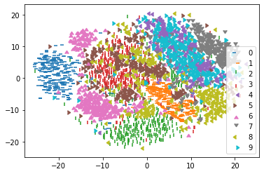
def scatter_plot(Y, labels):
    fig, ax = plt.subplots()
    for g in range(10):
        ix = np.where(labels == g)
        ax.scatter(Y[ix, 0], Y[ix, 1], label = g, marker = g, s = 30)
    ax.legend()
    plt.show()

def conditionalP(d2, beta, i):
    P = np.exp(-d2 * beta)
    Z = np.sum(P) - 1
    P = P / Z
    P[i] = 0
    return P

def computeP(D2):    
    n = D2.shape[0]
    conditionalPis = np.zeros((n, n))
    for i in range(n):
        beta = bisectBeta(D2[i, :])
        Pi = conditionalP(D2[i, :], beta, i)
        conditionalPis[i, :] = Pi
    Pij = (conditionalPis + conditionalPis.T) / (2 * n)
    Pij = np.maximum(Pij, 1e-12)
    return Pij

def computeQ(D2):
    n = D2.shape[0]
    Z = torch.sum(1. / (1 + D2)) - n
    Q = (1. / (1 + D2)) / Z
    Q = torch.clamp(Q, min=1e-12)
    return Q

def KL_divergence(P, Q):
    return torch.sum(P * torch.log(P / Q))

def tsne(X, labels, perplexity, lr, momentum = 0.9, max_iter = 1000, n_dim = 2, lambdal2 = 0.001, 
         pca_dim = 50, regularize_iter = 50, plot = True):
    X = pca(X, no_dims=pca_dim).real
    n = X.shape[0]
    Y = torch.distributions.Normal(0, 10**-4).sample((n, n_dim))
    Y.requires_grad = True
    xD2 = squaredDistanceMatrix(X)
    # early exaggeration
    P = torch.from_numpy(computeP(xD2)) * 4.
    optimizer = optim.SGD(params=[Y], lr=lr, momentum = momentum)
    
    for t in range(max_iter):
        optimizer.zero_grad()
        
        yD2 = squaredDistanceMatrix(Y)
        Q = computeQ(yD2)
        
        # early compression
        loss = KL_divergence(P, Q)
        if t < regularize_iter:
            loss = KL_divergence(P, Q) + lambdal2 * torch.sum(torch.square(Y))
        else:
            loss = KL_divergence(P, Q)
            
        loss.backward(retain_graph=True)
        optimizer.step()
        
        if (t + 1) % 50 == 0:
            print("Iteration {0}: KL-divergence is {1}".format(t + 1, loss))
            if plot:
                scatter_plot(Y.detach().numpy(), labels)
        
        # stop early exaggeration
        if (t + 1) == 100:
            P = P / 4.
        
    return Y

Load the MNIST dataset for t-SNE.

from scipy import io

mnist = io.loadmat('datasets/MNIST/train.mat')
mnist_img = np.transpose(mnist['train_images'], (2, 0, 1))
mnist_img = np.reshape(mnist_img, (mnist_img.shape[0], mnist_img.shape[1] * mnist_img.shape[2]))
mnist_label = mnist['train_labels']

shuffleIdx = np.random.choice(list(range(mnist_img.shape[0])), size = mnist_img.shape[0], replace = False)
mnist_img = mnist_img[shuffleIdx]
mnist_label = mnist_label[shuffleIdx]

mnist_img = mnist_img[:3000]
mnist_label = mnist_label[:3000]

Apply t-SNE.

Y = tsne(mnist_img, mnist_label, perplexity = 100, lr = 500, lambdal2 = 0.001, pca_dim = 300, 
         plot=False, max_iter = 300)

Iteration 50: KL-divergence is 13.574049788265157
Iteration 100: KL-divergence is 9.090292620655262
Iteration 150: KL-divergence is 0.8815392637246531
Iteration 200: KL-divergence is 0.8801887998921047
Iteration 250: KL-divergence is 0.8793375116145109
Iteration 300: KL-divergence is 0.8786649602861086

Visualize t-SNE results.

scatter_plot(Y.detach().numpy(), mnist_label)

References

1. Van der Maaten, Laurens, and Geoffrey Hinton. “Visualizing data using t-SNE.” Journal of machine learning research 9.11 (2008).
2. Goodfellow, Ian, et al. Deep learning. Vol. 1. No. 2. Cambridge: MIT press, 2016.