ResNet
1. Motivation
The following note introduces ResNet from the Deep Residual Learning for Image Recognition paper [1], which uses skip connections to enable easier optimization for deeper neural networks. The ResNet architecture was motivated by the degradation problem - adding more layers to an existing neural network leads to higher training error. Note this is a separate problem from overfitting or vanishing gradients. An example of this is illustrated by the figures below.

The authors argue that if a shallower architecture provides optimal mapping, then any extra layers added to it should learn the identity mapping. However, current optimization algorithms have a hard time learning the identity mapping, leading to increased training and test error. Thus, the ResNet architecture was developed to enable easier learning of identity mapping between layers.
2. Architecture
The following is the skip connection building block of the ResNet architecture, where the input activations are added elementwise to output activations a few layers later.

Assume for the above residual block that $\mathcal{H}(x)$ is the desired underlying mapping. However, $\mathcal{H}(x)$ may be difficult to find if for example, $\mathcal{H}(x) = x$. Instead, the layers of the residual block fits $\mathcal{F}(x)$, and outputs $\mathcal{H}(x) = \mathcal{F}(x) + x$ in the end. If $\mathcal{H}(x) = x$, then it is fairly easy to learn $\mathcal{F}(x) = 0$. For example, a fully-connected neural network simply has to set all weights and biases $W, b$ of the layers to 0 in order to achieve $\mathcal{F}(x) = 0$.
An implementation detail of the skip connection is to ensure $x$ and $\mathcal{F}(x)$ has the same dimensions. For a fully-connected residual block, dimension matching can be achieved by a learnable linear projection matrix $W_{s}$. Specifically, if $\mathcal{F}(x) \in \mathbb{R}^{m}$ and $x \in \mathbb{R}^{n}$, then the addition becomes $\mathcal{H}(x) = \mathcal{F}(x) + W_{s}x$ for $W_{s} \in \mathbb{R}^{m \times n}$. For convolution neural networks, without same convolution, the height, width, and number of channels between $\mathcal{F}(x)$ and $x$ may differ. In this case all dimensions are matched by running $x$ through a convolution with multiple $1 \times 1$ kernels. This is typically followed by batch normalization before addition to $\mathcal{F}(x)$.
3. Data Preparation
The dataset we will use is the CIFAR-10 [3] dataset, which contains 50,000 training images and 10,000 test images acrosss 10 classes, each of dimensions $32 \times 32 \times 3$. Our implementation of ResNet will use PyTorch 1.5.1. PyTorch utilities provide functions to output random mini-batches of data for training, which requires a Dataset class that loads and returns data.
import os
import torch
import torch.nn as nn
import torch.nn.functional as F
import pandas as pd
import numpy as np
from PIL import Image
import pickle
import torch.optim as optim
import matplotlib.pyplot as plt
from torch.utils.data import Dataset, DataLoader
from torch import utils
import torchvision.transforms as transforms
from torchsummary import summary
# Ignore warnings
import warnings
import math
warnings.filterwarnings("ignore")

class CIFAR10Dataset(Dataset):
    def __init__(self, data_dir, transform):
        #store filenames
        filenames = os.listdir(data_dir)
        filenames = [os.path.join(data_dir, f) for f in filenames]
        self.images, self.labels = [], []
        for f in filenames:
            image_batch, label_batch = self.__extract_reshape_file__(f)
            self.images = self.images + image_batch
            self.labels = self.labels + label_batch
        self.images = np.array(self.images)
        self.transform = transform

    def __extract_file__(self, fname):
        with open(fname, 'rb') as fo:
            d = pickle.load(fo, encoding='bytes')
        return d

    def __unflatten_image__(self, img_flat):
        img_R = img_flat[0:1024].reshape((32, 32))
        img_G = img_flat[1024:2048].reshape((32, 32))
        img_B = img_flat[2048:3072].reshape((32, 32))
        img = np.dstack((img_R, img_G, img_B))
        return img

    def __extract_reshape_file__(self, fname):
        d = self.__extract_file__(fname)
        images = []
        flattened_images, labels = d[b"data"], d[b"labels"]
        for i in range(len(flattened_images)):
            images.append(self.__unflatten_image__(flattened_images[i]))
        return images, labels

    def __len__(self):
        #return size of dataset
        return len(self.images)

    def __getitem__(self, idx):
        #apply transforms and return with label
        image = self.transform(self.images[idx])
        return image, self.labels[idx]

    def getUntransformedImage(self, idx):
        return self.images[idx], self.labels[idx]
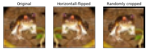
The data augmentation steps are:
- Randomly perform horizontal flip of image.
- Padding resulting image with 4 pixels on each side.
- Randomly crop $32 \times 32$ subimage from image.
transform = transforms.Compose([transforms.ToPILImage(),
                                transforms.RandomHorizontalFlip(),
                                transforms.RandomCrop(size = (32, 32),
                                                      padding = 4),
                                transforms.ToTensor()])

cifarDataset = CIFAR10Dataset("./data/cifar-10-batches-py/train", transform)
To visualize the augmentation effects.
import matplotlib.pyplot as plt
%matplotlib inline

ncol = 3
img, label = cifarDataset.getUntransformedImage(0)

# augmentation functions
horizontalFlip = transforms.Compose([transforms.ToPILImage(),
                                     transforms.RandomHorizontalFlip(p = 1.0)])
randomCrop = transforms.Compose([transforms.ToPILImage(),
                                 transforms.RandomCrop(size = (32, 32),
                                                       padding = 4)])

# perform augmentation
imgHorizontal = np.asarray(horizontalFlip(img))
imgCrop = randomCrop(img)

plt.figure(figsize=(2.2 * ncol, 2.2))
plt.subplots_adjust(bottom=0, left=.01, right=.99, top=.90, hspace=.20)

# original image
plt.subplot(1, ncol, 1)
plt.imshow(img)
plt.title("Original")
plt.xticks(())
plt.yticks(())

plt.subplot(1, ncol, 2)
plt.imshow(imgHorizontal)
plt.title("Horizontall-flipped")
plt.xticks(())
plt.yticks(())

plt.subplot(1, ncol, 3)
plt.imshow(imgCrop)
plt.title("Randomly cropped")
plt.xticks(())
# ";" added to suppress matplotlib message output
plt.yticks(());
Note that transforms.ToTensor() normalizes pixel values from range [0, 255] to range [0, 1]. Then split the non-test dataset into training and validation set. Following the ResNet paper, 5,000 images and labels will be set as validation dataset.
train_set, validation_set = utils.data.random_split(cifarDataset, [45000, 5000])
test_set = CIFAR10Dataset("./data/cifar-10-batches-py/test", transform)
4. Implementation
We implement a convolutional ResNet-20, largely following specifications described in “Section 4.2 CIFAR-10 and Analysis” of the ResNet paper. The components of the architecture are:
- Residual block.
- Layers comprised of $2n$ residual blocks (we choose $n = 3$).
- Multiple layers comprise the ResNet architecture.
As described in the paper, each layer is characterized by its number of filters and output map size. To reduce dimensions from one layer to the next, the first convolution of the first residual block of the next layer uses a stride of 2. The remaining convolutions in the layer are same convolutions.
class block(nn.Module):
    def __init__(self, in_channels, input_dim, channels, downsample_stride = 1,
                padding = 1, kernel_size = 3):
        super(block, self).__init__()
        self.input_dim = input_dim
        self.in_channels = in_channels
        self.channels = channels
        self.downsample_stride = downsample_stride
        self.padding = padding
        self.kernel_size = kernel_size
        self.__calc_output_size__()
        self.__initialize_graph_modules__()

    def __calc_output_size__(self):
        self.output_dim = math.floor((self.input_dim + 2 * self.padding - self.kernel_size) /\
                                     self.downsample_stride + 1)

    def __initialize_graph_modules__(self):
        self.bn = nn.BatchNorm2d(self.channels, track_running_stats = False)
        self.relu = nn.ReLU()

        # downsample conv layer
        self.conv1 = nn.Conv2d(self.in_channels, self.channels,
                               kernel_size = self.kernel_size,
                               padding = self.padding, stride=self.downsample_stride,
                               bias = False)
        # same conv layer
        self.conv2 = nn.Conv2d(self.channels, self.channels,
                               kernel_size = self.kernel_size,
                               padding = 1,
                               stride = 1,
                               bias = False)

        # identity shortcut
        if self.output_dim != self.input_dim:
            self.downsample = nn.Sequential(
                nn.Conv2d(self.in_channels, self.channels,
                          kernel_size = 1, stride = self.downsample_stride, bias=False,
                          padding = 0),
                nn.BatchNorm2d(self.channels, track_running_stats = False))
        else:
            self.downsample = None

    def forward(self, x):
        identity = x

        if self.downsample is not None:
            identity = self.downsample(identity)

        x = self.conv1(x)
        x = self.bn(x)
        x = self.relu(x)
        x = self.conv2(x)
        x += identity
        x = self.bn(x)
        x = self.relu(x)

        return x
Additonal selected implementation details are described below.
-
Weight initialization
- To stabilize variance of either activations or gradients for each layer, each weight value should be drawn from $\mathcal{N}(0, var)$, where $var$ is the appropriate variance specified by Kaiming et al. [2]
- $var$ depends on
- Stabilizing variance of activations (
fan_in) or variance of gradients (fan_out).fan_outis chosen. - Activation function is ReLU or PReLUs. ReLU is chosen.
- Stabilizing variance of activations (
- 2D Batch normalization
- Batch normalization is independently performed by channel.
- The batch normalization transformation is indicated below \(y = \frac{x - \bar{x}}{\sqrt{\hat{\sigma}(x) + \epsilon}}\gamma + \beta\) where $\bar{x}$ and $\hat{\sigma}(x)$ are empirical mean and variance respectively for a given mini-batch.
- The learnable scale and shift parameters $\gamma$ and $\beta$ are referred to as
weightandbiasby PyTorch, which are initialized to 1 and 0 respectively. - Canonical batch normalization keeps exponentially weighted averages of the $\bar{x}$ and $\hat{\sigma}(x)$ terms, then uses those statistics to perform normalization during inference. However, depending on the problem, using these statistics from training could degrade inference performance relative to using test mini-batch statistics. Experimentation suggests using test mini-batch statistics during inferences yields superior performance.
- Average pool 2D: applies 2D average pooling, which computes the average for each feature map.
class ResNet(nn.Module):
    def __init__(self, img_channels, learning_rate = 0.1, batch_size = 128,
                n = 3, num_classes = 10):
        # python2 compatible inheritance
        super(ResNet, self).__init__()
        self.batch_size = batch_size
        self.learning_rate = learning_rate
        self.img_channels = img_channels
        self.n = n
        self.num_classes = num_classes
        self.__initialize_graph_modules__()

    def __make_layer__(self, block, stride, in_channels, input_dim, channels):

        layers = []
        layers.append(block(in_channels, input_dim, channels, downsample_stride = stride))
        input_dim = math.floor((input_dim + 2 - 3) / stride + 1)

        for i in range(self.n - 1):
            layers.append(block(channels, input_dim, channels))

        return nn.Sequential(*layers)

    def __initialize_graph_modules__(self):
        self.conv1 = nn.Conv2d(self.img_channels, out_channels=16,
                               kernel_size=3, padding = 1)
        self.bn1 = nn.BatchNorm2d(16, track_running_stats = False)
        self.relu = nn.ReLU()

        # first block
        self.module1 = self.__make_layer__(block, stride=1, in_channels=16,
                                         input_dim=32, channels = 16)
        self.module2 = self.__make_layer__(block, stride=2, in_channels=16,
                                         input_dim=32, channels = 32)
        self.module3 = self.__make_layer__(block, stride=2, in_channels=32,
                                         input_dim=16, channels = 64)

        # fully connected
        self.avgpool = nn.AvgPool2d(kernel_size=(8, 8))
        self.fc = nn.Linear(in_features=64, out_features=self.num_classes)
        self.softmax = nn.Softmax()

        # initialize weights
        for m in self.modules():
            if isinstance(m, nn.Conv2d):
                nn.init.kaiming_normal_(m.weight, mode='fan_out', nonlinearity='relu')
            elif isinstance(m, nn.BatchNorm2d):
                nn.init.constant_(m.weight, 1)
                nn.init.constant_(m.bias, 0)

    def forward(self, x):
        x = self.conv1(x)
        x = self.bn1(x)
        x = self.relu(x)
        x = self.module1(x)
        x = self.module2(x)
        x = self.module3(x)
        x = self.avgpool(x)
        x = torch.flatten(x, start_dim = 1)
        x = self.fc(x)
        return x

    def predict_probabilities(self, x):
        x = self.forward(x)
        return self.softmax(x)

    def predict_class(self, x):
        x = self.forward(x)
        return torch.argmax(self.softmax(x), dim = 1)
View a summary of model weights.
device = torch.device("cuda" if torch.cuda.is_available() else "cpu")
resnet = ResNet(img_channels=3).to(device)

summary(resnet, input_size=(3, 32, 32))
----------------------------------------------------------------
        Layer (type)               Output Shape         Param #
================================================================
            Conv2d-1           [-1, 16, 32, 32]             448
       BatchNorm2d-2           [-1, 16, 32, 32]              32
              ReLU-3           [-1, 16, 32, 32]               0
            Conv2d-4           [-1, 16, 32, 32]           2,304
       BatchNorm2d-5           [-1, 16, 32, 32]              32
              ReLU-6           [-1, 16, 32, 32]               0
            Conv2d-7           [-1, 16, 32, 32]           2,304
       BatchNorm2d-8           [-1, 16, 32, 32]              32
              ReLU-9           [-1, 16, 32, 32]               0
            block-10           [-1, 16, 32, 32]               0
           Conv2d-11           [-1, 16, 32, 32]           2,304
      BatchNorm2d-12           [-1, 16, 32, 32]              32
             ReLU-13           [-1, 16, 32, 32]               0
           Conv2d-14           [-1, 16, 32, 32]           2,304
      BatchNorm2d-15           [-1, 16, 32, 32]              32
             ReLU-16           [-1, 16, 32, 32]               0
            block-17           [-1, 16, 32, 32]               0
           Conv2d-18           [-1, 16, 32, 32]           2,304
      BatchNorm2d-19           [-1, 16, 32, 32]              32
             ReLU-20           [-1, 16, 32, 32]               0
           Conv2d-21           [-1, 16, 32, 32]           2,304
      BatchNorm2d-22           [-1, 16, 32, 32]              32
             ReLU-23           [-1, 16, 32, 32]               0
            block-24           [-1, 16, 32, 32]               0
           Conv2d-25           [-1, 32, 16, 16]             512
      BatchNorm2d-26           [-1, 32, 16, 16]              64
           Conv2d-27           [-1, 32, 16, 16]           4,608
      BatchNorm2d-28           [-1, 32, 16, 16]              64
             ReLU-29           [-1, 32, 16, 16]               0
           Conv2d-30           [-1, 32, 16, 16]           9,216
      BatchNorm2d-31           [-1, 32, 16, 16]              64
             ReLU-32           [-1, 32, 16, 16]               0
            block-33           [-1, 32, 16, 16]               0
           Conv2d-34           [-1, 32, 16, 16]           9,216
      BatchNorm2d-35           [-1, 32, 16, 16]              64
             ReLU-36           [-1, 32, 16, 16]               0
           Conv2d-37           [-1, 32, 16, 16]           9,216
      BatchNorm2d-38           [-1, 32, 16, 16]              64
             ReLU-39           [-1, 32, 16, 16]               0
            block-40           [-1, 32, 16, 16]               0
           Conv2d-41           [-1, 32, 16, 16]           9,216
      BatchNorm2d-42           [-1, 32, 16, 16]              64
             ReLU-43           [-1, 32, 16, 16]               0
           Conv2d-44           [-1, 32, 16, 16]           9,216
      BatchNorm2d-45           [-1, 32, 16, 16]              64
             ReLU-46           [-1, 32, 16, 16]               0
            block-47           [-1, 32, 16, 16]               0
           Conv2d-48             [-1, 64, 8, 8]           2,048
      BatchNorm2d-49             [-1, 64, 8, 8]             128
           Conv2d-50             [-1, 64, 8, 8]          18,432
      BatchNorm2d-51             [-1, 64, 8, 8]             128
             ReLU-52             [-1, 64, 8, 8]               0
           Conv2d-53             [-1, 64, 8, 8]          36,864
      BatchNorm2d-54             [-1, 64, 8, 8]             128
             ReLU-55             [-1, 64, 8, 8]               0
            block-56             [-1, 64, 8, 8]               0
           Conv2d-57             [-1, 64, 8, 8]          36,864
      BatchNorm2d-58             [-1, 64, 8, 8]             128
             ReLU-59             [-1, 64, 8, 8]               0
           Conv2d-60             [-1, 64, 8, 8]          36,864
      BatchNorm2d-61             [-1, 64, 8, 8]             128
             ReLU-62             [-1, 64, 8, 8]               0
            block-63             [-1, 64, 8, 8]               0
           Conv2d-64             [-1, 64, 8, 8]          36,864
      BatchNorm2d-65             [-1, 64, 8, 8]             128
             ReLU-66             [-1, 64, 8, 8]               0
           Conv2d-67             [-1, 64, 8, 8]          36,864
      BatchNorm2d-68             [-1, 64, 8, 8]             128
             ReLU-69             [-1, 64, 8, 8]               0
            block-70             [-1, 64, 8, 8]               0
        AvgPool2d-71             [-1, 64, 1, 1]               0
           Linear-72                   [-1, 10]             650
================================================================
Total params: 272,490
Trainable params: 272,490
Non-trainable params: 0
----------------------------------------------------------------
Input size (MB): 0.01
Forward/backward pass size (MB): 5.16
Params size (MB): 1.04
Estimated Total Size (MB): 6.21
----------------------------------------------------------------
5. Training
We train the Adam optimization algorithm with random mini-batches with each epoch. The train settings are
- Maximum of 50 epochs.
- If validation accuracy does not improve consecutively over five 50 mini-batches, then terminate training.
def calculate_accuracy(model, validationloader):
    model.eval()
    for data in validationloader:
        imgs, labels = data
    predictions = model.predict_class(imgs)
    predictions = predictions.numpy()
    labels = labels.numpy()
    model.train()
    return np.mean(predictions == labels)

trainloader = torch.utils.data.DataLoader(train_set, batch_size=128, shuffle=True)
validationloader = torch.utils.data.DataLoader(validation_set, batch_size=5000, shuffle=False)

printStr = "[epoch {:d}, batch {:d}]: running train cross entropy: {:.3f} | validation accuracy: {:.3f}"
earlyStop = False
earlyStopThreshold = 5
nonIncreaseCounter = 0
prevValAccuracy = -float('inf')
maxEpochs = 50
optimizer = optim.Adam(params=resnet.parameters(), lr=0.001, weight_decay=0.0001)
criterion = nn.CrossEntropyLoss()

for epoch in range(maxEpochs):
    if earlyStop:
        break
    running_loss = 0.0
    for i, data in enumerate(trainloader, 1):
        imgs, labels = data

        optimizer.zero_grad()

        outputs = resnet(imgs)
        loss = criterion(outputs, labels)
        loss.backward()
        optimizer.step()

        running_loss += loss.item()
        # print every 50 mini-batches
        if i % 50 == 0:
            valAccuracy = calculate_accuracy(resnet, validationloader)
            print(printStr.format(epoch + 1, i, running_loss / 50, valAccuracy))
            running_loss = 0.0

            if valAccuracy <= prevValAccuracy:
                nonIncreaseCounter += 1
            else:
                nonIncreaseCounter = 0
            prevValAccuracy = valAccuracy

            if nonIncreaseCounter > earlyStopThreshold:
                earlyStop = True
                break
Select output
[epoch 1, batch 50]: running train cross entropy: 2.074 | validation accuracy: 0.288
[epoch 1, batch 100]: running train cross entropy: 1.756 | validation accuracy: 0.349
[epoch 1, batch 150]: running train cross entropy: 1.645 | validation accuracy: 0.390
[epoch 1, batch 200]: running train cross entropy: 1.575 | validation accuracy: 0.431
[epoch 1, batch 250]: running train cross entropy: 1.495 | validation accuracy: 0.452
[epoch 1, batch 300]: running train cross entropy: 1.390 | validation accuracy: 0.495
[epoch 1, batch 350]: running train cross entropy: 1.321 | validation accuracy: 0.520
[epoch 2, batch 50]: running train cross entropy: 1.269 | validation accuracy: 0.545
[epoch 2, batch 100]: running train cross entropy: 1.225 | validation accuracy: 0.544
[epoch 2, batch 150]: running train cross entropy: 1.212 | validation accuracy: 0.565
[epoch 2, batch 200]: running train cross entropy: 1.178 | validation accuracy: 0.583
[epoch 2, batch 250]: running train cross entropy: 1.182 | validation accuracy: 0.595
[epoch 2, batch 300]: running train cross entropy: 1.118 | validation accuracy: 0.603
[epoch 2, batch 350]: running train cross entropy: 1.114 | validation accuracy: 0.609
Save the model and optimizer parameters.
torch.save({'model_state_dict': resnet.state_dict(),
           'optimizer_state_dict': optimizer.state_dict()},
          "./models/resnet.pt")
6. Evaluation
Load the model weights.
resnet_saved = ResNet(img_channels=3)
checkpoint = torch.load("./models/resnet.pt")
resnet_saved.load_state_dict(checkpoint['model_state_dict'])
_ = resnet_saved.eval()
Evaluate test accuracy.
testloader = torch.utils.data.DataLoader(test_set, batch_size=10000, shuffle=False)
test_accuracy = calculate_accuracy(resnet_saved, testloader)

print("test accuracy: {0}".format(test_accuracy))
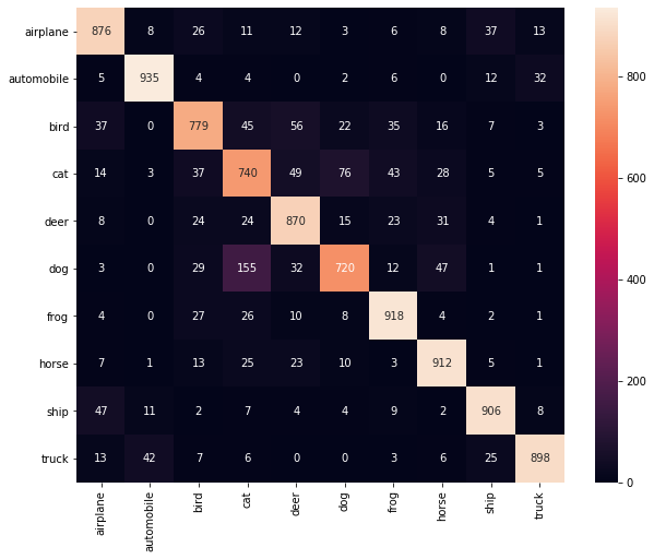
test accuracy: 0.8578
Plot confusion matrix.
from sklearn.metrics import confusion_matrix
import seaborn as sn
import pandas as pd

with open("data/cifar-10-batches-py/batches.meta", 'rb') as fo:
    meta_data = pickle.load(fo, encoding='bytes')

for data in testloader:
    testImg, testlabel = data

testlabel = testlabel.numpy()
pred_class = resnet_saved.predict_class(testImg)

confusion_matix = confusion_matrix(testlabel, pred_class)
class_names = [s.decode("utf-8") for s in meta_data[b'label_names']]
df_cm = pd.DataFrame(confusion_matix, index = class_names, columns=class_names)
plt.figure(figsize=(10, 8))
sn.heatmap(df_cm, annot = True, fmt='d')
Reference
- He, Kaiming, et al. “Deep residual learning for image recognition.” Proceedings of the IEEE conference on computer vision and pattern recognition. 2016.
- He, Kaiming, et al. “Delving deep into rectifiers: Surpassing human-level performance on imagenet classification.” Proceedings of the IEEE international conference on computer vision. 2015.
- Krizhevsky, Alex, and Geoffrey Hinton. “Learning multiple layers of features from tiny images.” (2009): 7.