Generative Adversarial Network

1. Introduction

Generative adversarial network (GAN) is a framework for learning to represent an estimate $p_{\text{model}}$ of the distribution $p_{\text{data}}$ from its samples. The standard GAN estimates $p_{\text{data}}$ implicitly by being able to generate samples from $p_{\text{model}}$. In contrast, explicit estimation requires a defined density function $p_{\text{model}}(x; \theta)$.

The main idea behind how GANs learn is through a game between a generator and a discriminator. The generator’s goal is to learn to generate samples from the same distribution as the training data. The discriminator’s goal is to learn to discriminate between fake generated samples and true training samples. Both players optimize the same value function $V(D, G)$, but only with respect to their own parameters (from $D$ or $G$). The solution to this game is referred to as a local differential Nash equilibria, a point in the parameter space where all neighboring points have less than or equal value. After training, the generator is used to generate samples that may aesthetically appear similar to samples from the training data. The following post is based on the original GAN paper as well as the NIPS 2016 tutorial on GANs [1, 2].

2. Method

Let the generator $G$ and discriminator $D$ be parameterized by neural networks. GANs learn by having $G$ and $D$ play the following minimax game

\[\min_{G}\max_{D}V(D, G) = \min_{G}\max_{D}\mathbb{E}_{x \sim p_{\text{data}}(x)}[\log D(x)] + \mathbb{E}_{z \sim p_{z}(z)}[\log(1 - D(G(z)))],\]

where $p_{z}(z)$ is a prior distribution of input noise variables. The generator learns a mapping from $z$ to the data space. The discriminator $D(x) \in [0, 1]$ outputs a probability that an input sample comes from $p_{\text{data}}$ rather than the generator’s distribution $p_{g}$. This game is a zero-sum game because if $\max_{D}V(D, G)$ is re-expressed as minimizing a cost $\min_{D}-V(D, G) = \min_{D}J^{(D)}$, then $\min_{G}V(D, G) = \min_{G}J^{(G)}$ implies $J^{(G)} = -J^{(D)}$. Zero-sum games are alternatively called minimax games.

Intuitively, \(\max_{D}\mathbb{E}_{x \sim p_{\text{data}}(x)}[\log D(x)]\) maximizes the log-probability of the discriminator being correct on real samples, and \(\max_{D}\mathbb{E}_{z \sim p_{z}(z)}[\log(1 - D)]\) maximizes the log-probability of being correct on fake samples, because \(\arg\max_{D \in [0, 1]}\log(1 - D) = 0\). For $G$, \(\min_{G}V(D, G)\) amounts to minimizing the log-probability of the discriminator being correct ($D(G(z)) = 1$) since \(\arg\min_{D \in [0, 1]}\log(1 - D) = 1\).

2.1 Optimal Discriminator

For a given $G$, $\arg\max_{D}V(D, G) = \frac{p_{\text{data}}}{p_{\text{data}} + p_{g}}$. This is determined by solving for $D$ such that

\[\frac{\partial}{\partial D}V(D, G) = 0\]

for every given $x$. To start, rewrite $V(D, G)$ in terms of $p_{\text{data}}$ and $p_{g}$

\[\begin{align*} V(D, G) &= \mathbb{E}_{x \sim p_{data}}[\log D(x)] + \mathbb{E}_{z \sim p_{z}(z)}[\log(1 - D(G(z)))]\\ &= \int_{x \in \mathcal{X}}\log D(x) p_{\text{data}}(x)dx + \int_{z \in \mathcal{Z}}\log(1 - D(G(z)))p_{z}(z)dz\\ &= \int_{x \in \mathcal{X}}\log D(x) p_{\text{data}}(x)dx + \int_{x \in \mathcal{X}}\log(1 - D(x))p_{g}(x)dx\\ &= \int_{x \in \mathcal{X}}\log D(x) p_{\text{data}}(x) + \log(1 - D(x))p_{g}(x)dx, \end{align*}\]

where in the third step, we apply the law of the unconscious statistician with \(\mathbb{E}_{z}[G(z)] = \mathbb{E}_{x}[x]\) for $x = G(z)$. Then

\[\begin{align*} \frac{\partial V(D, G)}{\partial D(x)} = \frac{p_{\text{data}}(x)}{D(x)} - \frac{p_{g}(x)}{1 - D(x)} = 0 \Rightarrow D^{*}(x) = \frac{p_{\text{data}}(x)}{p_{g}(x) + p_{\text{data}}(x)}. \end{align*}\]

2.2 Optimal Generator

Define $C(G) = \max_{D}V(G, D)$, then global minimum of $C(G)$ is achieved if and only if $p_{g} = p_{\text{data}}$. At that point, $C(G)$ achieves the value $-\log 4$. We will first show that $\min C(G) = -\log 4$. Start by adding and subtracting $-\log 4$ to $C(G) = V(G, D^{*})$

\[\begin{align*} C(G) &= -\log 4 +2\log 2 + \mathbb{E}_{x \sim p_{\text{data}}(x)}\left[\log \frac{p_{\text{data}}(x)}{p_{\text{data}}(x) + p_{g}(x)}\right] + \mathbb{E}_{x \sim p_{g}}\left[\log \frac{p_{g}(x)}{p_{\text{data}}(x) + p_{g}(x)}\right]\\ &= -\log 4 + \mathbb{E}_{x \sim p_{\text{data}}(x)}[\log 2] + \mathbb{E}_{x \sim p_{g}}[\log 2] + \mathbb{E}_{x \sim p_{\text{data}}(x)}\left[\log \frac{p_{\text{data}}(x)}{p_{\text{data}}(x) + p_{g}(x)}\right]\\ &\quad + \mathbb{E}_{x \sim p_{g}}\left[\log \frac{p_{g}(x)}{p_{\text{data}}(x) + p_{g}(x)}\right]\\ &= -\log 4 + \mathbb{E}_{x \sim p_{\text{data}}(x)}\left[\log \frac{2p_{\text{data}}(x)}{p_{\text{data}}(x) + p_{g}(x)}\right] + \mathbb{E}_{x \sim p_{g}}\left[\log \frac{2p_{g}(x)}{p_{\text{data}}(x) + p_{g}(x)}\right]\\ &= -\log 4 + KL\left(p_{\text{data}}(x) \bigg\lvert \bigg\lvert \frac{p_{\text{data}}(x) + p_{g}(x)}{2}\right) + KL\left(p_{g}(x) \bigg\lvert \bigg\lvert \frac{p_{\text{data}}(x) + p_{g}(x)}{2} \right)\\ &= -\log 4 + \underbrace{2 JSD(p_{\text{data}} \lvert \lvert p_{g})}_{\geq 0}, \end{align*}\]

since Jensen-Shannon divergence $JSD(p_{\text{data}} \lvert \lvert p_{g}) \geq 0$, $\min_{G}C(G) = -\log 4$.

To prove that $\min_{G}C(G) = -\log 4 \Leftrightarrow p_{g} = p_{\text{data}}$. When $p_{g} = p_{\text{data}}$, $JSD(p_{\text{data}} \lvert\lvert p_{g}) = 0$, the minimum value of $C(G) = -\log 4$ is achieved. When $C(G) = -\log 4$, this implies $JSD(p_{\text{data}} \lvert\lvert p_{g}) = 0$ and $p_{\text{data}} = p_{g}$.

In other words, an optimal generator learns the distribution of the data completely.

2.3 Heuristic, non-saturating game

The value function $V(D, G)$ is useful for theoretical analysis but does not perform well in practice. In the initial training iterations, the discriminator tends to reject generator samples with high confidence, and this causes the generator’s gradient to vanish. Concretely, when $D$ rejects samples from $G(z)$ with high confidence, $D(G(z)) \approx 0$. This leads to \(\log (1) = 0 \Rightarrow \mathbb{E}_{z \sim p_{z}(z)}[\log(1 - D(G(z)))] = 0\), so the gradient with respect to generator weights will be zero.

The heuristic game addresses this by having the generator minimize \(-\mathbb{E}_{z \sim p_{z}(z)}\log D(G(z))\) instead, which corresponds to maximizing the log-probability of the discriminator being mistaken. In this version of the game, the game is no longer zero-sum.

3. Implementation

We will implement a GAN to generate realistic-looking images. Since the input data are images, the generator and discriminator are chosen to be parameterized by convolutional neural networks. This type of GAN is called the deep convolutional generative adversarial network (DCGAN) [3]. Our implementation of a DCGAN in PyTorch 1.5.1 will largely following the one presented by this resource. The diagram below illustrates the architecture of a DCGAN.

Following the resource, we will also apply the DCGAN to the LWF Face Dataset, which consists of 13,000 images of faces. First download the dataset.

import os
import wget
import tarfile

lfw_url = 'http://vis-www.cs.umass.edu/lfw/lfw-deepfunneled.tgz'
data_path = 'data'

wget.download(lfw_url, data_path + "/lfw.tgz")
# extract compressed files
with tarfile.open(data_path + "/lfw.tgz") as tar:
    tar.extractall(path = data_path)

'data/lfw.tgz'

We first create a Dataset class that loads and returns this data. Following Radford and Chintala [3], we normalize the pixel values to $[-1, 1]$, the range of the tanh activation function.

import os
import torch
import torch.nn as nn
import torch.nn.functional as F
import pandas as pd
import numpy as np
from PIL import Image
import pickle
import matplotlib.pyplot as plt
import torch.optim as optim
import matplotlib.pyplot as plt
from torch.utils.data import Dataset, DataLoader
from torch import utils
import torchvision.transforms as transforms
from torchsummary import summary
import torchvision.utils as vutils
# Ignore warnings
import warnings
import math
warnings.filterwarnings("ignore")

class LWFDataset(Dataset):
    def __init__(self, data_dir, width = 64, height = 64):      
        # load data
        self.width = width
        self.height = height
        self.images = []
        for path, _, fnames in os.walk(data_dir):
            for fname in fnames:
                if not fname.endswith('.jpg'):
                    continue
                filepath = os.path.join(path, fname)
                img = plt.imread(filepath)
                self.images.append(img)
        self.images = np.array(self.images)
        self.toPIL = transforms.Compose([transforms.ToPILImage()])
        self.toTensor = transforms.Compose([transforms.ToTensor()])
        
    def transform(self, img):
        img = self.toPIL(img)
        img = transforms.functional.resize(img, (self.height, self.width))
        img = np.array(img)
        #img = np.transpose(np.array(img), (2, 0, 1))
        # normalize to [-1, 1]
        img = img.astype(np.float32) / 127.5 - 1
        # if image is greyscale, repeat 3 times to get RGB image.
        if img.shape[0] == 1:
            img = np.tile(img, (3, 1, 1))
        return img

    def __len__(self):
        #return size of dataset
        return len(self.images)

    def __getitem__(self, idx):
        #apply transforms and return with label
        image = self.transform(self.images[idx])
        return self.toTensor(image)
    
    def getUntransformedImage(self, idx):
        return self.images[idx]

Download dataset.

lwfDataset = LWFDataset('data/lfw-deepfunneled')
dataloader = torch.utils.data.DataLoader(lwfDataset, batch_size=128, shuffle=True)

Following the architecture guidelines for stable DCGANs

• Replace any pooling layers with strided convolutions (discriminator) and fractional-strided convolutions (generator).
• Use batch normalization in both the generator and the discriminator.
• Remove fully connected hidden layers for deeper architectures.
• Use ReLU activation in generator for all layers except for the output, which uses Tanh (so that output range equals input range of normalized pixel values).
• Use LeakyReLU activation in the discriminator for all layers.

We will first implement the generator. The first layer is a “project and reshape” layer, which we implement as a linear, fully-connected layer, to project the input $z \in \mathbb{R}^{100 \times 1 \times 1}$ into a vector in $\mathbb{R}^{8192}$ space, which then gets reshaped into a tensor of shape $\mathbb{R}^{512 \times 4 \times 4}$. The remaining layers are 2D transpose convolution layers for projection into higher dimensional spaces.

class Generator(nn.Module):
    def __init__(self, z = 100, imgDim = 64, nc = 3):
        super(Generator, self).__init__()
        self.imgDim = imgDim
        self.z = z
        self.nc = nc
        self.__initialize_graph__()
        self.__initialize_weights__()
        
    def __initialize_graph__(self):
        self.main = nn.Sequential(
            # transpose Conv1
            nn.ConvTranspose2d(in_channels=self.imgDim * 8, out_channels=self.imgDim * 4, 
                               kernel_size=4, stride=2, padding=1, bias=False),
            nn.BatchNorm2d(num_features=self.imgDim * 4),
            nn.ReLU(inplace=True),
            # transpose Conv2
            nn.ConvTranspose2d(in_channels=self.imgDim * 4, out_channels=self.imgDim * 2, 
                               kernel_size=4, stride=2, padding=1, bias=False),
            nn.BatchNorm2d(num_features=self.imgDim * 2),
            nn.ReLU(inplace=True),
            # transpose Conv3
            nn.ConvTranspose2d(in_channels=self.imgDim * 2, out_channels=self.imgDim, 
                               kernel_size=4, stride=2, padding=1, bias=False),
            nn.BatchNorm2d(num_features=self.imgDim),
            nn.ReLU(inplace=True),
            # transpose Conv4
            nn.ConvTranspose2d(in_channels=self.imgDim, out_channels=self.nc, 
                               kernel_size=4, stride=2, padding=1, bias=False),
            # G(z)
            nn.Tanh()        
        )
        self.project = nn.Linear(in_features=self.z, out_features=self.imgDim * 128, bias=True)
        
    def __initialize_weights__(self):
        for m in self.modules():
            if isinstance(m, nn.ConvTranspose2d):
                nn.init.normal_(m.weight, mean=0, std=0.2)
            elif isinstance(m, nn.BatchNorm2d):
                nn.init.normal_(m.weight, 1, 0.02)
                nn.init.constant_(m.bias, 0)
    
    def forward(self, x):
        # project and reshape
        x = torch.flatten(x, start_dim=1)
        x = self.project(x)
        x = x.view(x.shape[0], 512, 4, 4)
        # transpose convolutions
        return self.main(x)

Create an instance of generator and view summary of it.

device = torch.device("cuda" if torch.cuda.is_available() else "cpu")
netG = Generator().to(device)
summary(netG, input_size=(100, 1, 1))

----------------------------------------------------------------
        Layer (type)               Output Shape         Param #
================================================================
            Linear-1                 [-1, 8192]         827,392
   ConvTranspose2d-2            [-1, 256, 8, 8]       2,097,152
       BatchNorm2d-3            [-1, 256, 8, 8]             512
              ReLU-4            [-1, 256, 8, 8]               0
   ConvTranspose2d-5          [-1, 128, 16, 16]         524,288
       BatchNorm2d-6          [-1, 128, 16, 16]             256
              ReLU-7          [-1, 128, 16, 16]               0
   ConvTranspose2d-8           [-1, 64, 32, 32]         131,072
       BatchNorm2d-9           [-1, 64, 32, 32]             128
             ReLU-10           [-1, 64, 32, 32]               0
  ConvTranspose2d-11            [-1, 3, 64, 64]           3,072
             Tanh-12            [-1, 3, 64, 64]               0
================================================================
Total params: 3,583,872
Trainable params: 3,583,872
Non-trainable params: 0
----------------------------------------------------------------
Input size (MB): 0.00
Forward/backward pass size (MB): 2.88
Params size (MB): 13.67
Estimated Total Size (MB): 16.55
----------------------------------------------------------------

We implement the discriminator with the following features:

• Strided convolution in place of pooling to allow network to learn its own pooling function.
• Batch normalization and leaky ReLU to promote healthy gradient flow.

class Discriminator(nn.Module):
    def __init__(self, imgDim=64, nc=3, ndf=64):
        super(Discriminator, self).__init__()
        self.imgDim = imgDim
        self.nc = nc
        self.ndf = ndf
        self.__initialize_graph__()
        self.__initialize_weights__()
        
    def __initialize_graph__(self):
        self.main = nn.Sequential(
            # Conv1
            nn.Conv2d(in_channels=self.nc, out_channels=self.ndf, kernel_size=4, 
                      stride=2, padding=1, bias=False),
            nn.LeakyReLU(negative_slope=0.2, inplace=True),
            # Conv2
            nn.Conv2d(in_channels=self.ndf, out_channels=self.ndf * 2, 
                      kernel_size=4, stride=2, padding=1, bias=False),
            nn.BatchNorm2d(num_features=self.ndf * 2),
            nn.LeakyReLU(negative_slope=0.2, inplace=True),
            # Conv3
            nn.Conv2d(in_channels=self.ndf * 2, out_channels=self.ndf * 4, 
                      kernel_size=4, stride=2, padding=1, bias=False),
            nn.BatchNorm2d(num_features=self.ndf * 4),
            nn.LeakyReLU(negative_slope=0.2, inplace=True),
            # Conv4
            nn.Conv2d(in_channels=self.ndf * 4, out_channels=self.ndf * 8, 
                      kernel_size=4, stride=2, padding=1, bias=False),
            nn.BatchNorm2d(num_features=self.ndf * 8),
            nn.LeakyReLU(negative_slope=0.2, inplace=True),
            # Conv5
            nn.Conv2d(in_channels=self.ndf * 8, out_channels=1, 
                      kernel_size=4, stride=1, padding=0, bias=False),
            nn.Sigmoid()
        )
        
    def __initialize_weights__(self):
        for m in self.modules():
            if isinstance(m, nn.Conv2d):
                nn.init.normal_(m.weight, mean=0, std=0.2)
            elif isinstance(m, nn.BatchNorm2d):
                nn.init.normal_(m.weight, 1, 0.02)
                nn.init.constant_(m.bias, 0)
    
    def forward(self, x):
        return self.main(x)

Create an instance of discriminator and view summary of it.

netD = Discriminator().to(device)
summary(netD, input_size=(3, 64, 64))

----------------------------------------------------------------
        Layer (type)               Output Shape         Param #
================================================================
            Conv2d-1           [-1, 64, 32, 32]           3,072
         LeakyReLU-2           [-1, 64, 32, 32]               0
            Conv2d-3          [-1, 128, 16, 16]         131,072
       BatchNorm2d-4          [-1, 128, 16, 16]             256
         LeakyReLU-5          [-1, 128, 16, 16]               0
            Conv2d-6            [-1, 256, 8, 8]         524,288
       BatchNorm2d-7            [-1, 256, 8, 8]             512
         LeakyReLU-8            [-1, 256, 8, 8]               0
            Conv2d-9            [-1, 512, 4, 4]       2,097,152
      BatchNorm2d-10            [-1, 512, 4, 4]           1,024
        LeakyReLU-11            [-1, 512, 4, 4]               0
           Conv2d-12              [-1, 1, 1, 1]           8,192
          Sigmoid-13              [-1, 1, 1, 1]               0
================================================================
Total params: 2,765,568
Trainable params: 2,765,568
Non-trainable params: 0
----------------------------------------------------------------
Input size (MB): 0.05
Forward/backward pass size (MB): 2.31
Params size (MB): 10.55
Estimated Total Size (MB): 12.91
----------------------------------------------------------------

Now we implement the training procedure. Following recommendation from the 2016 GAN tutorial [2], we implement one-sided label smoothing, which prevents extreme extrapolation behavior. In other words, label smoothing prevents the discriminator from predicting extremely large logits. This helps the discriminator converge to $D^{*}(x) = \frac{p_{\text{data}}(x)}{p_{g}(x) + p_{\text{data}}(x)}$.

# Initialize binary cross entropy function
criterion = nn.BCELoss()

# Create batch of latent vectors that we will use to visualize
#  the progression of the generator
fixed_noise = torch.randn(128, 100, 1, 1)

# Establish convention for real and fake labels during training
real_label = 0.9
fake_label = 0.

# Setup Adam optimizers for both G and D
optimizerD = optim.Adam(netD.parameters(), lr=0.0002, betas=(0.5, 0.999))
optimizerG = optim.Adam(netG.parameters(), lr=0.0002, betas=(0.5, 0.999))

A few notes on implementation details

• For some reason $z \sim \mathcal{N}(0, I)$ performs better compared to $z_{i} \sim Unif(0, 1)$ for $i = 1, \dots ,100$.
• When computing discriminator gradient, call .detach() for generated images so that gradient with respect to generator weights will not be computed.

# Training Loop
img_list = []
G_losses = []
D_losses = []
iters = 0

# Lists to keep track of progress
num_epochs = 100

print("Starting Training Loop...")
# For each epoch
for epoch in range(num_epochs):
    # For each batch in the dataloader
    for i, data in enumerate(dataloader, 0):

        ############################
        # (1) Update D network: maximize log(D(x)) + log(1 - D(G(z)))
        ###########################
        ## Train with all-real batch
        netD.zero_grad()
        # Format batch
        b_size = data.size()[0]
        label = torch.full((b_size,), real_label, dtype=torch.float)
        # Forward pass real batch through D
        output = netD(data).view(-1)
        # Calculate loss on all-real batch
        errD_real = criterion(output, label)
        # Calculate gradients for D in backward pass
        errD_real.backward()
        D_x = output.mean().item()

        ## Train with all-fake batch
        # Generate batch of latent vectors
        noise = torch.randn(b_size, nz, 1, 1)
        # Generate fake image batch with G
        fake = netG(noise)
        label.fill_(fake_label)
        # Classify all fake batch with D
        output = netD(fake.detach()).view(-1)
        # Calculate D's loss on the all-fake batch
        errD_fake = criterion(output, label)
        # Calculate the gradients for this batch
        errD_fake.backward()
        D_G_z = output.mean().item()
        # Add the gradients from the all-real and all-fake batches
        errD = errD_real + errD_fake
        # Update D
        optimizerD.step()

        ############################
        # (2) Update G network: maximize log(D(G(z)))
        ###########################
        netG.zero_grad()
        label.fill_(real_label)  # fake labels are real for generator cost
        # Since we just updated D, perform another forward pass of all-fake batch through D
        output = netD(fake).view(-1)
        # Calculate G's loss based on this output
        errG = criterion(output, label)
        # Calculate gradients for G
        errG.backward()
        # Update G
        optimizerG.step()

        # Output training stats
        if i % 5 == 0:
            print('[%d/%d][%d/%d]\tLoss_D: %.4f\tLoss_G: %.4f\tD(x): %.4f\tD(G(z)): %.4f'
                  % (epoch, num_epochs, i, len(dataloader),
                     errD.item(), errG.item(), D_x, D_G_z))

        # Save Losses for plotting later
        G_losses.append(errG.item())
        D_losses.append(errD.item())

        # Check how the generator is doing by saving G's output on fixed_noise
        if (iters % 500 == 0) or ((epoch == num_epochs-1) and (i == len(dataloader)-1)):
            with torch.no_grad():
                fake = netG(fixed_noise).detach().cpu()
            img_list.append(vutils.make_grid(fake, padding=2, normalize=True))

        iters += 1

Sample training output messages

Starting Training Loop...
[0/20][0/104]	Loss_D: 1.4444	Loss_G: 5.3994	D(x): 0.9483	D(G(z)): 0.4281
[0/20][5/104]	Loss_D: 1.3202	Loss_G: 3.9553	D(x): 0.9328	D(G(z)): 0.3406
[0/20][10/104]	Loss_D: 1.0306	Loss_G: 4.3411	D(x): 0.8991	D(G(z)): 0.2811
[0/20][15/104]	Loss_D: 1.0606	Loss_G: 2.9521	D(x): 0.8990	D(G(z)): 0.3044
[0/20][20/104]	Loss_D: 1.1041	Loss_G: 2.1576	D(x): 0.6295	D(G(z)): 0.1640
[0/20][25/104]	Loss_D: 1.6851	Loss_G: 1.2120	D(x): 0.3495	D(G(z)): 0.0336
[0/20][30/104]	Loss_D: 1.3260	Loss_G: 1.7409	D(x): 0.4221	D(G(z)): 0.0491
[0/20][35/104]	Loss_D: 1.0421	Loss_G: 2.4594	D(x): 0.5918	D(G(z)): 0.1079
[0/20][40/104]	Loss_D: 1.1397	Loss_G: 4.1079	D(x): 0.5686	D(G(z)): 0.0549
[0/20][45/104]	Loss_D: 0.7310	Loss_G: 5.0861	D(x): 0.8848	D(G(z)): 0.1409

4. Results

Visualize the progression of the generated images from the same input noise $z$.

import matplotlib.animation as animation
from IPython.display import HTML

fig = plt.figure(figsize=(20,10))
plt.axis("off")
ims = [[plt.imshow(np.transpose(i,(1,2,0)), animated=True)] for i in img_list]
ani = animation.ArtistAnimation(fig, ims, interval=1000, repeat_delay=1000, blit=True)

HTML(ani.to_jshtml())

</input>

Once Loop Reflect

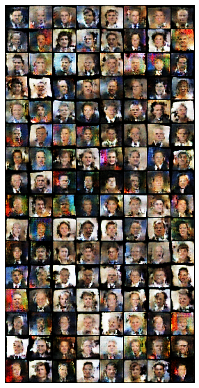
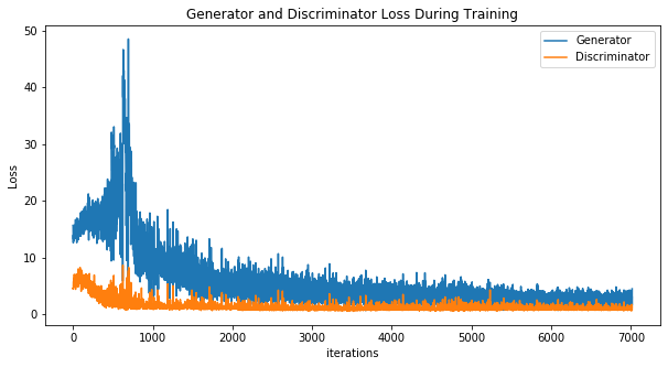
Visualize the generator and discriminator loss over iterations of training batches. Both generator and discriminator loss show some degree of convergence behavior. From experiment, aesthetically more pleasing images are generated when the discriminator starts off with low loss, and the generator tries to “catch up” by generating more similar images to the training images. In contrast, when the discriminator starts off with high loss and the generator with low loss, the generator appears unable to generate aesthetically pleasing images with roughly same number of iterations.

plt.figure(figsize=(10,5))
plt.title("Generator and Discriminator Loss During Training")
plt.plot(G_losses,label="Generator")
plt.plot(D_losses,label="Discriminator")
plt.xlabel("iterations")
plt.ylabel("Loss")
plt.legend()
plt.show()

References

1. Goodfellow, Ian, et al. “Generative adversarial nets.” Advances in neural information processing systems. 2014.
2. Goodfellow, Ian. “NIPS 2016 tutorial: Generative adversarial networks.” arXiv preprint arXiv:1701.00160 (2016).
3. Radford, Alec, Luke Metz, and Soumith Chintala. “Unsupervised representation learning with deep convolutional generative adversarial networks.” arXiv preprint arXiv:1511.06434 (2015).