Optimal Stopping
1. The Secretary Problem
1.1 Introduction
The secretary problem is the problem of finding the best candidate to hire out of $n$ rankable candidates from a sequence of 1-on-1 interviews, in random order. A hiring decision is made after each interview, with each decision being irreversible - any reject or hire decision is final. Wikipedia and Christian and Griffiths [1] introduce more useful details, and the key problem formulations are reproduced below for convenience:
- There is a clear ranking of $n$ candidates, with $n$ known in advance. Only the relative ranking is known.
- Each sequence of $n$ interviews is equally likely.
- After an interview, a candidate must be either rejected or accepted. Once a hiring decision is made, the interview loop ends.
- A hiring decision can only be made based on the quality of candidates interviewed thus far.
The problem asks for an algorithm for determining where in the interview loop to make a hiring decision in order to maximize the probability of hiring the best candidate. Intuitively, hiring the first candidate encountered may be a bad idea because it is helpful to first establish a baseline of candidate quality first. However, waiting until the last candidate may be a bad idea because the best candidate has likely already been passed. It turns out the optimal algorithm is to reject the first $r - 1 = n / e$ applicants, noting the best applicant $M$ from this pool. Then, the first subsequent applicant better than $M$ is accepted. This maximizes the probability of hiring the best candidate, which stands at $1 / e$.
The optimal algorithm at first appears useful for many common real-life scenarios that resemble the secretary problem, such as apartment search and hiring. However, a skeptical friend of mine rightfully pointed out that many real-life hiring scearios do not resemble the secretary problem exactly. For example, some hiring decisions are not made right after an interview. Following this line of thought, the assumptions that $n$ is known and that the ordering of candidate interviews is random may be too strong as well. Lastly, how practically-relevant is a success probability guarantee if the candidate search is performed once? This blog post attempts to address some of these limitations.
1.2 Deriving the Optimal Algorithm
We start by deriving the optimal algorithm for the secretary problem. Under the premise to
- Reject the first $r - 1$ applicants, noting best applicant $M$
- Accept the subsequent applicant better than $M$,
we derive the probability of selecting the best candidate $P(r)$ that is dependent on $r$. This derivation is largely based on the one provided by wikipedia.
\[\begin{align*} P(r) &= \sum_{i = 1}^{n}P(\text{applicant $i$ is selected $\cap$ applicant $i$ is the best})\\ &= \sum_{i = 1}^{n}P(\text{applicant $i$ is selected $\lvert$ applicant $i$ is the best})\cdot P(\text{applicant $i$ is the best})\\ &= \left[\sum_{i = 1}^{r - 1}0 + \sum_{i = r}^{n}P(\text{best of first $i - 1$ applicants among first $r - 1$ applicant $\lvert$ applicant $i$ is best})\right] \cdot \frac{1}{n}\\ &= \left[\sum_{i = r}^{n}\frac{r - 1}{i - 1}\right]\cdot \frac{1}{n}\\ &= \frac{r - 1}{n}\sum_{i = r}^{n}\frac{1}{i - 1}. \end{align*}\]We break down the third line. The sum of the first $r - 1$ terms is zero since the first $r - 1$ applicants are rejected, by construction. The marginal probability that applicant $i$ is the best is simply $1/n$ by the random ordering assumption. Finally, the conditional probability term is due to the fact that if applicant $i$ is the best, then it is selected if and only if the best applicant among the first $i - 1$ applicants is among the first $r - 1$ applicants rejected. We prove both the forward statement and its converse for this fact. Assuming applicant $i$ is best,
- If applicant $i$ is selected by the algorithm, then $i > M$ (short for candidate $i$ is better than candidate $M$) and $r,\dots,i - 1 < M$. Since $M > 1, \dots ,r - 1$ by definition, this implies that the best of the first $i - 1$ applicants is $M$, which is also among first $r - 1$ applicants rejected.
- Define $M^{\prime}$ to be best candidate among first $i - 1$ candidates. Then if $M^{\prime}$ is also among first $r - 1$ candidates rejected, then the algorithm will not accept any of the candidates $r, \dots ,i - 1$, by definition of $M^{\prime}$. Since applicant $i$ is the best applicant and is the first applicant better than $M^{\prime}$, the algorithm will choose $i$.
The conditional probability $P(\text{best of first $i - 1$ applicants among first $r - 1$ applicant $\lvert$ applicant $i$ is best}) = \frac{r - 1}{i - 1}$ is again due to the assumption that any interview sequence is equally likely. In other words, conditional on selection of candidate $i$, $M^{\prime}$ can only fall in the first $i - 1$ positions. Out of the $i - 1$ equally likely positions candidate $M^{\prime}$ can be in, only the first $r - 1$ of those positions correspond to the event that the best of first $i - 1$ candidates is among the first $r - 1$ rejected.
We next rewrite $P(r)$ using a series of mathematical manipulations to observe what happens when $n, r \rightarrow \infty$ (largely based on this math stackexchange post).
\[\begin{align*} P(r) &= \frac{r - 1}{n}\sum_{i = r}^{n}\frac{1}{i - 1}\\ &= \frac{r - 1}{n}\sum_{i = r - 1}^{n - 1}\frac{1}{i}\\ &= \frac{r - 1}{n}\left(\frac{1}{r - 1} + \sum_{i = r}^{n - 1}\frac{1}{i}\right)\\ &= \frac{1}{n} + \frac{r - 1}{n}\left(\sum_{i = 1}^{n - 1}\frac{1}{i} - \sum_{i = 1}^{r - 1}\frac{1}{i}\right)\\ &= \frac{1}{n} + \frac{r - 1}{n}\left(\sum_{i = 1}^{n}\frac{1}{i} - \log(n - 1) - \left(\sum_{i = 1}^{r - 1}\frac{1}{i} - \log(r - 1)\right)\right) + \frac{r - 1}{n}\log\frac{n - 1}{r - 1} \end{align*}\]Since both $n, r$ are whole numbers with $r < n$, we can re-write $\frac{r - 1}{n} = x + O(n)$, where $O(n) \rightarrow 0$ as $n \rightarrow \infty$. For example, if $r = \lfloor 1 + nx \rfloor$, then $x - \frac{1}{n} < \frac{r - 1}{n} \leq x$. By squeeze theorem, since $\lim_{n \rightarrow \infty} x - \frac{1}{n} = x$ and $\lim_{n \rightarrow \infty}x = x$, we have $\lim_{n \rightarrow \infty}\frac{r - 1}{n} = x$. Now substitue $\frac{r - 1}{n} = x + O(n)$ into the last expression above to get
\[\begin{align*} P(r) &= \frac{1}{n} + (x + O(n))\left(\sum_{i = 1}^{n}\frac{1}{i} - \log(n - 1) - \left(\sum_{i = 1}^{r - 1}\frac{1}{i} - \log(r - 1)\right)\right) + (x + O(n))\log\frac{1 - 1/n}{x + O(n)}. \end{align*}\]Take $n \rightarrow \infty$ and $r \rightarrow \infty$ and apply the Euler–Mascheroni constant fact that $\lim_{m \rightarrow \infty}\sum_{i = 1}^{m}\frac{1}{i} - \log m = \gamma$ to arrive at
\[\begin{align*} \lim_{n, r \rightarrow \infty}&\frac{1}{n} + (x + O(n))\left(\sum_{i = 1}^{n}\frac{1}{i} - \log(n - 1) - \left(\sum_{i = 1}^{r - 1}\frac{1}{i} - \log(r - 1)\right)\right) + (x + O(n))\log\frac{1 - 1/n}{x + O(n)}\\ =& x(\gamma - \gamma) - x\log x. \end{align*}\]Now that we can express probability of selecting the best candidate as $P(x) = -x\log x$, we can determine $x^{\ast} = \arg\max_{x} P(x)$ as
\[\begin{align*} \frac{dP(x)}{dx} = -\log x - 1 = 0 \Rightarrow x^{\ast} = \frac{1}{e}, \end{align*}\]which is optimal because $d^{2} P(x) / d x^{2} = -\frac{1}{x} < 0$ for $x \in [0, 1)$. Hence, as $n \rightarrow \infty$, the best $r - 1$ approaches $n / e$ to achieve an optimal success probability of $P(x^{\ast}) = 1 / e \approx 0.3679$.
1.3 Simulation
How does a success probability $P(r)$ translate in a real-life application? After all, after an interview loop ends, the only possible outcomes are failure or success in hiring the best candidate. First notice that $P(r) = \mathbb{E}[\mathbb{1}(\text{best candidate is hired})]$, which is an expectation. The weak law of large numbers states that as the number of trials $m$ approaches infinity, the average approaches the expected value. More technically, we have the following convergence in probability
\[\bar{X} \stackrel{P}{\rightarrow} \mu\]where $\bar{X} = \frac{1}{n}\sum_{i = 1}^{n}x_{i}$ and $\mu = \mathbb{E}[X]$. Thus, what a success probability guarantee really tells us is that if the set of $n$ interviews is repeatedly multiple times according to the optimial stopping algorithm, the proportion of times the best candidate is selected is around 37.79%.
Let us study this via a simulation generating a random sequence of rankable candidates. We have control over two parameters:
- The number of candidates $n$.
- The number of trials $m$ that the interview loop involving $n$ candidates is repeated.
Based on the derivation above, both $m$ and $n$ need to be large for the proportion of best candidate hires to be close to the 37.79%. We test values $n = 10$ and $n = 100$, which could correspond to apartment search and hiring in real-life scenarios. Then, we vary $m$ from 1 to 1,000, and observe how the running success proportion varies.
import numpy as np

def generateCandidateSeq(n):
    return np.random.permutation(n)

def optimalStopping(candidates):
    n = len(candidates)
    r = int(n / np.exp(1) + 1)
    M = -np.inf

    # observe best candidate M
    for i in range(r - 1):
        if candidates[i] > M:
            M = candidates[i]

    # return first candidate better than M
    r = r - 1
    while r < n and candidates[r] < M:
        r += 1
    if r == n:
        return r - 1
    return r

def simulation(m, n):
    prop = 0
    for i in range(m):
        candidates = generateCandidateSeq(n)
        decision = optimalStopping(candidates)
        if candidates[decision] == n - 1:
            prop += 1
    return prop / float(m)
Now run the simulation for $n = 10$ and $n = 100$ for $m = 1, \dots ,1000$.
mList = list(range(1, 1001, 10))
props10 = []
props100 = []

for m in mList:
    props10.append(simulation(m, 10))
    props100.append(simulation(m, 100))
Plot results.
import matplotlib.pyplot as plt
%matplotlib inline

fig, ax = plt.subplots(figsize=(12, 6))
ax.plot(mList, props10, 'o-', markersize = 2, color = "blue", label = "n = 10")
ax.plot(mList, props100, 'o-', markersize = 2, color = "red", label = "n = 100")
ax.set_xlabel('Number of trials', fontsize=16)
ax.set_ylabel('Proportion success', fontsize=16)
ax.tick_params(axis='both', which='major', labelsize=16)
ax.legend(fontsize=16)
plt.show()
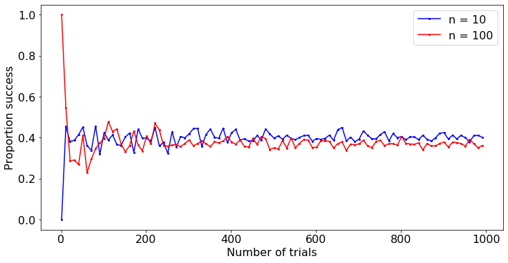
For both $n = 10, 100$, we see the running success proportions converge to a value just under 40%. At $m = 1,000$, is the success proportion for $n = 10$ or $n = 100$ closer to 0.3679?
print("Absolute difference with 36.79% (n = 10): {0}".format(abs(props10[-1] - 0.3679)))
print("Absolute difference with 36.79% (n = 100): {0}".format(abs(props100[-1] - 0.3679)))
Absolute difference with 36.79% (n = 10): 0.033714530776992935
Absolute difference with 36.79% (n = 100): 0.006648738647830499
As expected, the success proportion for $n = 100$ is closer to the expected success proportion of 0.3679.
2. When to Sell
2.1 Introduction
Imagine selling a house where
- Offers are made sequentially, with an accept or reject decision required after each offer.
- You know the minimum and maximum possible offers $O_{\min}$ and $O_{\max}$ based on knowledge of the market.
- All offers in your offer range is equally likely.
- Waiting for another offer incurs a fixed cost $r$ (e.g. mortgage payment).
This variant was introduced by Christian and Griffiths [1]. In this scenario, the optimal policy is to not sell until an offer is made beyond a pre-determined minimum threshold $t \in [O_{\min}, O_{\max}]$. What threshold $t$ should we select? While you can wait until an offer close to the maximum possible is made, such offers also require longer wait times, which incur higher cost. The answer is to find $t$ such that the expected gain from taking an offer better than $t$ is at least the expected cost of waiting until an offer better than $t$ is made. Why does this make sense? Because this guarantee means that on average, the gain from waiting for a good offer outstrips the cost of waiting.
2.2 Deriving the Optimal Sell Threshold
Define
- $W_{t}$: number of waits before a better offer than $t$ is made.
- $G_{t}$: gain from taking offer better than $t$.
- $C_{t}$: cost of waiting until offer better than $t$. Given $W_{t}$, $C_{t} = W_{t}r$.
For any $t$, define profit as $P_{t} = G_{t} - C_{t}$. Finally, define the optimization problem as
\[\begin{align*} \max_{t \in [O_{\min}, O_{\max}]}&t\\ \mathbb{E}[P_{t}] &\geq 0. \end{align*}\]In other words, the objective is to maximize the minimum acceptance threshold $t$ while ensuring that the expected gain is at least the expected cost of waiting.
We start by explicitly computing $\mathbb{E}[P_{t}] = \mathbb{E}[G] - \mathbb{E}[C]$. The gain is the conditional expectation $\mathbb{E}[G] = \mathbb{E}[\text{offer} \lvert \text{offer better than $t$}]$. Since any offer is equally likely, the conditional expectation can be explicitly computed as
\[\begin{align*} \mathbb{E}[\text{offer} \lvert \text{offer better than $t$}] &= \int_{0}^{O_{\max} - t}\frac{o}{O_{\max} - t}do\\ &= \frac{1}{2(O_{\max} - t)}[o^{2}]_{0}^{O_{\max} - t}\\ &= \frac{O_{\max} - t}{2}. \end{align*}\]On the other hand, the number of waits $W_{t}$ follows a geometric distribution parameterized by $p_{t}$, the probability that an offer better than $t$ is made. Again, due to each offer being equally likely, $p_{t} = \frac{O_{\max} - t}{O_{\max} - O_{\min}}$. Since $C_{t} = W_{t}r$,
\[\mathbb{E}[C_{t}] = r\mathbb{E}[W_{t}] = \frac{r}{p_{t}} = \frac{r(O_{\max} - O_{\min})}{O_{\max} - t},\]where we use the fact that $\mathbb{E}[W_{t}] = \frac{1}{p_{t}}$.
All the remains is to find $t$, and we start by examining the $\mathbb{E}[P_t]$ versus $t$ curve. The slope is given by
\[\frac{d\mathbb{E}[P_{t}]}{dt} = -\left(\frac{1}{2} + \frac{r(O_{\max} - O_{\min})}{(O_{\max} - t)^{2}}\right) < 0,\]which tells us that the curve is monotonically decreasing on $t \in [O_{\min}, O_{\max}]$. To illustrate, let $O_{\max} = 500,000$, $O_{\min} = 400,000$, and $r = 2000$
def expectedProfit(oMax, oMin, r, t):
    return (oMax - t) / 2 - (r * (oMax - oMin)) / (oMax - t)

oMin = 400000
oMax = 500000
r = 2000

thresholds = list(range(401000, 500000, 1000))
eProfits = [expectedProfit(oMax, oMin, r, t) for t in thresholds]

fig, ax = plt.subplots(figsize=(12, 6))
ax.plot(thresholds, eProfits, 'o-', markersize = 2, color = "blue")
ax.set_xlabel('Offer acceptance threshold t', fontsize=16)
ax.set_ylabel('Expected profit', fontsize=16)
ax.tick_params(axis='both', which='major', labelsize=16)
plt.show()
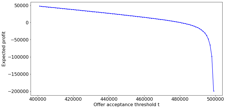
From examining $d\mathbb{E}[P_{t}] / dt$ and the plot above, we can reason that maximum $t$ under the constraint that $\mathbb{E}[P_{t}] \geq 0$ occurs when $t$ takes on the value such that $\mathbb{E}[P_{t}] = 0$.
\[\begin{align*} \mathbb{E}[P_{t}] &= 0 \iff \frac{O_{\max} - t}{2} = \frac{r(O_{\max} - O_{\min})}{O_{\max} - t}\\ &\iff t^{2} - 2tO_{\max} + O_{\max}^{2} - 2r(O_{\max} - O_{\min}) = 0\\ &\iff t^{\ast} = O_{\max} - \sqrt{2r(O_{\max} - O_{\min})} \end{align*}\]Finally, we can plot the offer threshold $t$ versus wait cost $r$ curve.
def getThreshold(Omin, Omax, r):
    return Omax - np.sqrt(2 * r * (Omax - Omin))

Omin, Omax = 400000, 500000
rs = list(range(1, 50001, 1000))
thresholds = [getThreshold(Omin, Omax, r) for r in rs]

fig, ax = plt.subplots(figsize=(12, 6))
ax.plot(rs, thresholds, 'o-', markersize = 2, color = "blue")
ax.set_xlabel('Cost per offer r', fontsize=16)
ax.set_ylabel('Offer threshold t', fontsize=16)
ax.tick_params(axis='both', which='major', labelsize=16)
plt.show()
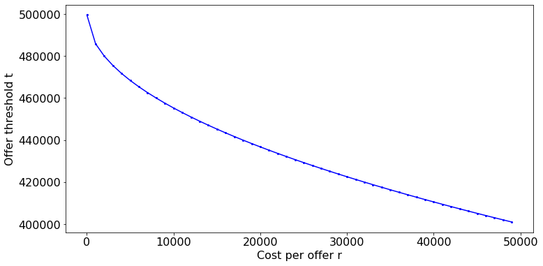
When the cost of waiting is big, you have less luxury of waiting for a good offer from the market.
3. When to Stop
3.1 Introduction
Imagine a game where each round you stand to win reward $r$ with success probability $p$, but also stand to lose all of your cumulated rewards with probability $1 - p$. Given you have succeeded up to $n$ rounds, when should you stop? This game has often been introduced as the “burglar problem”, where each round is a robbery that can either end of success or with getting caught.
More formally, given $n$ successful robberies with cumulated reward $nr$, does robbing or quitting maximize the expected cumulative reward on the next round? It turns out we can solve for $n$ such that if the burglar succeeds for $n$ consecutive rounds, he or she should quit.
3.2 Deriving the Optimal Stopping Threshold
After $n$ successful rounds, the burglar decides to rob or quit based on maximizing the expected cumulative reward on the next round
\[R(n) = \max(nr, p(n + 1)r),\]where the $nr$ is the expected reward of quitting and $p(n + 1)r$ is the expected reward of robbing. Rewrite $P(n) = p(n + 1)r - nr$ as the gain in expected reward if a robbery is made in the next round. Thus, the optimal decision is to rob if $P(n) > 0$. We can analyze the $P(n)$ versus $n$ curve by examining the first derivative
\[\frac{dP(n)}{dn} = r(p - 1) < 0,\]which indicates $P(n)$ decreases monotonically with $n$. Thus, we should continue to rob until $P(n) = 0$. Solving for $n$ such that $P(n) = 0$
\[\begin{align*} P(n) &= p(n + 1)r - nr = 0\\ &\Rightarrow n(rp - r) = -pr\\ &\Rightarrow n^{\ast} = \frac{p}{1 - p}. \end{align*}\]For example, if you have a success rate of 90%, you should quit after successfully robbing 9 times.
References
- Christian, Brian, and Tom Griffiths. Algorithms to live by: The computer science of human decisions. Macmillan, 2016.