Locally-Weighted Logistic Regression
1. Introduction
The following note is based on contents of Stanford’s CS229 public course. Given a query point/test point $x \in \mathbb{R}^{n}$ and $m$ training data points, the maximization objective of locally-weighted logistic regression is
\[\ell(\theta) = -\frac{\lambda}{2}\theta^{\top}\theta + \sum_{i = 1}^{m}w^{(i)}\left[y^{(i)}\log h_{\theta}(x^{(i)}) + (1 - y^{(i)})\log (1 - h_{\theta}(x^{(i)}))\right],\]where
- Training point $i$ is $x^{(i)} \in \mathbb{R}^{n}$ with label $y^{(i)} \in {0, 1}$.
- Regularization parameter $\lambda \in \mathbb{R}$.
- Model weights are $\theta \in \mathbb{R}^{n}$.
- $h_{\theta}(x) = \frac{1}{1 + \exp(-x^{\top}\theta)}$, the sigmoid function.
- Weight $w^{(i)} = \text{exp}\left(-\frac{\lvert\lvert x - x^{(i)} \lvert \lvert^{2}}{2\tau^{2}}\right)$ weights the influence of each training datapoint $x^{(i)}$ on $\theta$.
We can search for optimal weights $\theta^{*}$ via the Newton-Raphson algorithm, which is a second-order optimization algorithm
\[\theta := \theta - H^{-1}\nabla_{\theta}\ell(\theta),\]where $H \in \mathbb{R}^{n \times n}$ is the hessian of $\ell(\theta)$ with respect to $\theta$.
2. Derivation
We derive the explicit expression for the Newton-Raphson update. Start with the gradient term $\nabla_{\theta}\ell(\theta)$. Since $h_{\theta}(z) = \sigma(z)$, the sigmoid function, it is a fact that $\frac{d\sigma(z)}{dz} = \sigma(z) (1 - \sigma(z))$.
\[\frac{\partial \log \sigma(\theta^{\top}x^{(i)})}{\partial \theta_{j}} = \frac{1}{\sigma(\theta^{\top}x^{(i)})}\sigma(\theta^{\top}x^{(i)}) (1 - \sigma(\theta^{\top}x^{(i)}))x_{j}^{(i)} = (1 - \sigma(\theta^{\top}x^{(i)}))x_{j}^{(i)}\] \[\frac{\partial \log (1 - \sigma(\theta^{\top}x^{(i)}))}{\partial \theta_{j}} = - \frac{\sigma(\theta^{\top}x^{(i)})}{1 - \sigma(\theta^{\top}x^{(i)})}(1 - \sigma(\theta^{\top}x^{(i)}))x_{j}^{(i)} = -\sigma(\theta^{\top}x^{(i)})x_{j}^{(i)}\]Using the above results,
\[\begin{align*} \frac{\partial \ell(\theta)}{\partial \theta_{j}} &= -\lambda \theta_{j} + \sum_{i = 1}^{m}x_{j}^{(i)}w^{(i)}(y^{(i)} - h_{\theta}(x^{(i)})) \Rightarrow \nabla_{\theta}\ell(\theta) = -\lambda \theta + X^{\top}W(y - h_{\theta}(x)) \end{align*}\]where $X \in \mathbb{R}^{m \times n}$ is the training dataset matrix, \(W = diag(\{w^{(i)}\}_{i = 1}^{m}) \in \mathbb{R}^{m \times m}\), and $y, h_{\theta}(x) \in \mathbb{R}^{m}$. To find the Hessian,
\[\frac{\partial^{2} \ell(\theta)}{\partial \theta_{j} \partial \theta_{k}} = -\lambda \mathbb{1}(j = k) - \sum_{i = 1}^{m}x_{j}^{(i)}w^{(i)}h_{\theta}(x^{(i)})(1 - h_{\theta}(x^{(i)}))x_{k}^{(i)} \Rightarrow H = X^{\top}DX - \lambda I_{n},\]where $D \in \mathbb{R}^{m \times m}$ is a diagonal matrix with
\[D_{ii} = -w^{(i)}h_{\theta}(x^{(i)})(1 - h_{\theta}(x^{(i)}))\]3. Implementation
Load libraries and sample datasets.
import numpy as np
import pandas as pd
import pylab as pl
from matplotlib.colors import ListedColormap
import matplotlib.pyplot as plt

DATA_DIR = "datasets/CS229_P1"
X = pd.DataFrame(np.loadtxt(DATA_DIR + "/x.dat"))
Y = pd.DataFrame(np.loadtxt(DATA_DIR + "/y.dat"))
Below is implementation of locally-weighted logistic regression using the Newton-Raphson optimization method.
class locally_weighted_logistic_regression(object):

    def __init__(self, tau, reg = 0.0001, threshold = 1e-6):
        self.reg = reg
        self.threshold = threshold
        self.tau = tau
        self.w = None
        self.theta = None
        self.x = None

    def weights(self, x_train, x):
        sq_diff = (x_train - x)**2
        norm_sq = sq_diff.sum(axis = 1)
        return np.ravel(np.exp(- norm_sq / (2 * self.tau**2)))

    def logistic(self, x_train):
        return np.ravel(1 / (1 + np.exp(-x_train.dot(self.theta))))

    def train(self, x_train, y_train, x):
        self.w = self.weights(x_train, x)
        self.theta = np.zeros(x_train.shape[1])
        self.x = x
        gradient = np.ones(x_train.shape[1]) * np.inf
        while np.linalg.norm(gradient) > self.threshold:
            # compute gradient
            h = self.logistic(x_train)
            gradient = x_train.T.dot(self.w * (np.ravel(y_train) - h)) - self.reg * self.theta
            # Compute Hessian
            D = np.diag(-(self.w * h * (1 - h)))
            H = x_train.T.dot(D).dot(x_train) - self.reg * np.identity(x_train.shape[1])
            # weight update
            self.theta = self.theta - np.linalg.inv(H).dot(gradient)

    def predict(self):
        return np.array(self.logistic(self.x) > 0.5).astype(int)
4. Evalulation
Evaluate the behavior of the model’s classification boundary at bandwith parameters $\tau = 0.05, 0.1, 0.5, 1$
def plot_lwlr(x_train, y_train, tau, res):
    lwlr = locally_weighted_logistic_regression(tau)
    # Setup plotting grid
    xx, yy = np.meshgrid(np.linspace(-1, 1, res), np.linspace(-1, 1, res))
    cmap_light = ListedColormap(['#FFAAAA', '#AAFFAA'])
    cmap_bold = ListedColormap(['#FF0000', '#00FF00'])
    # Make predictions
    x = np.zeros(2)
    pred = np.zeros((res, res))
    for i in range(res):
        for j in range(res):
            x[0] = xx[i, j]
            x[1] = yy[i, j]
            lwlr.train(x_train, y_train, x)
            pred[i, j] = lwlr.predict()
    # Plotting
    plt.figure()
    plt.pcolormesh(xx, yy, pred, cmap=cmap_light)
    plt.scatter(x_train.iloc[:, 0], x_train.iloc[:, 1], c = y_train.iloc[:, 0],
                cmap=cmap_bold)
    plt.xlabel("x")
    plt.ylabel("y")
    plt.axis("tight")
    plt.title("tau = " + str(tau))
    plt.gca().set_aspect('equal', adjustable='box')
    plt.show()
Plots below.
%matplotlib inline
tau = [0.05, 0.1, 0.5, 1]

for i in range(1, len(tau) + 1):

    plot_lwlr(X, Y, tau[i-1], 50)
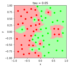
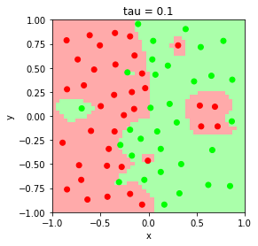
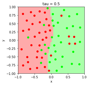
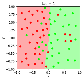
The parameter $\tau$ is related to the weight according to
\[w^{(i)} = \exp\left(-\frac{||x - x^{(i)}||^{2}}{2\tau^{2}}\right).\]Smaller $\tau$ values result in high variance, low bias decision boundary, and larger $\tau$ values result in low variance, high bias decision boundary. As $\tau \rightarrow \infty$, $w^{(i)} \rightarrow 1$, and the model converges to unweighted logistic regression.