Multiple Hypothesis Testing
1. Motivation
It is important to control for false discoveries when multiple hypotheses are tested. Under the Neyman-Pearson formulation, each hypothesis test involves a decision rule with false positive rate (FPR) less than $\alpha$ (e.g. $\alpha = 0.05$). However, if there are $m$ $\alpha$-level independent tests, the probability of at least one false discovery could be as high as $\min(m\alpha, 1)$. Multiple hypothesis testing correction involves adjusting the significance level(s) to control error related to false discoveries. Some of the material presented is based on UC Berkeley’s Data102 course.
2. P-values
Consider $H_{0}: \theta = \theta_{0}$ versus $H_{1}: \theta = \theta_{1}$. Let \(\mathbb{P}_{\theta_{0}}(x)\) be the distribution of data \(X \in \mathbb{R}^{p}\) under the null, and let \(S = \{X^{(i)}\}_{i = 1}^{m}\) be the observed dataset. Additionally, denote $S_{0}$ as the unobserved dataset drawn from \(\mathbb{P}_{\theta_{0}}(x)\).
If the statistic $T(S_{0})$ has tail cumulative distribution function (CDF) \(F(t) = \mathbb{P}_{\theta_{0}}(T(S_{0}) > t)\), then the p-value is defined as the random variable $P = F(T(S))$. The graphical illustration of the density of $T$ (short for $T(S)$) is shown below.
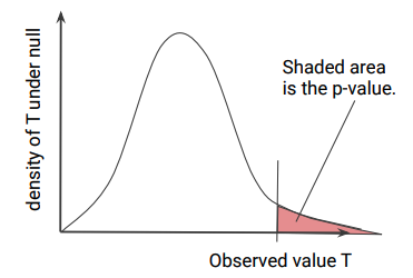
An important fact about p-value $P$ is that it has $Unif(0, 1)$ distribution under the null. A random variable has $Unif(0, 1)$ distribution if and only if it has CDF $F(p) = p$ for $p \in [0, 1]$. We now show $P$ has CDF $F(p) = p$.
\[\mathbb{P}_{\theta_{0}}(P \leq p) = \mathbb{P}_{\theta_{0}}(F(T) \leq p) = \mathbb{P}_{\theta_{0}}(T > F^{-1}(p)) = F(F^{-1}(p)) = p\]where the first equality is by definition of $P$. For the second equality, it is helpful to recall that for the 1-to-1 function $F(\cdot)$, $F: T \rightarrow u$ and $F^{-1}: u \rightarrow T$. Then from diagram above, notice that $F(T)$ is decreasing with respect to $T$. The third equality is from definition of $F(\cdot)$.
3. Bonferroni Correction
Let $V$ be the number of false positives. Then the probability of at least one false discovery $V > 0$ among $m$ tests (not necessarily independent) is defined as the family-wise error rate (FWER). Bonferroni correction adjusts the significance level to $\alpha / m$. This controls the FWER to be at most $\alpha$. If there are $m_{0} \leq m$ true null hypotheses, then
\[\begin{align*} \text{FWER} = \mathbb{P}\left(\bigcup_{i = 1}^{m_{0}}\big\{P_{i} \leq \frac{\alpha}{m}\big\}\right) \leq \sum_{i = 1}^{m_{0}}\mathbb{P}\left(P_{i} \leq \frac{\alpha}{m}\right) = m_{0}\frac{\alpha}{m} \leq m\frac{\alpha}{m} = \alpha, \end{align*}\]where the first inequality is from union bound (Boole’s inequality). In practice, the observed p-value $p_{i}$ is adjusted according to
\[p_{i}^{adj} = \min\{mp_{i}, 1\}\]for $i = 1, \dots, m$. Then the $i$-th null hypothesis is rejected if $p_{i}^{adj} \leq \alpha$. Let us simulate 10 p-values from $unif(0, 0.3)$ and implement Bonferroni corrected p-values.
from statsmodels.stats.multitest import multipletests
import numpy as np

# simulation
n = 10
pvals = np.random.uniform(0, 0.3, size = n)

# implementation of Bonferroni correction
def bonferroni(pvals):
    m = len(pvals)
    return sorted([round(m * p, 7) if m * p <= 1 else 1 for p in pvals])

pAdj1 = bonferroni(pvals)
_, pAdj2, _, _ = multipletests(pvals, method = "bonferroni", returnsorted = True)

print(pAdj1)
print(pAdj2)
[0.0677386, 0.1100421, 0.5649019, 0.7202574, 0.7341066, 1, 1, 1, 1, 1]
[0.06773857 0.11004206 0.56490188 0.72025737 0.7341066  1.
 1.         1.         1.         1.        ]
4. Benjamini-Hochberg
A major criticism of Bonferroni correction is that it is too conservative - false positives are avoided at the expense of false negatives. The Benjamini-Hochberg (BH) procedure instead controls the FDR to avoid more false negatives. The FDR among $m$ tests is defined as
\[FDR = \mathbb{E}\left[\frac{V}{R}\right]\]where $R$ is number of rejections among $m$ tests. BH procedure adjusts the p-value cutoff by allowing looser p-value cutoffs provided given earlier discoveries. This is graphically illustrated below.
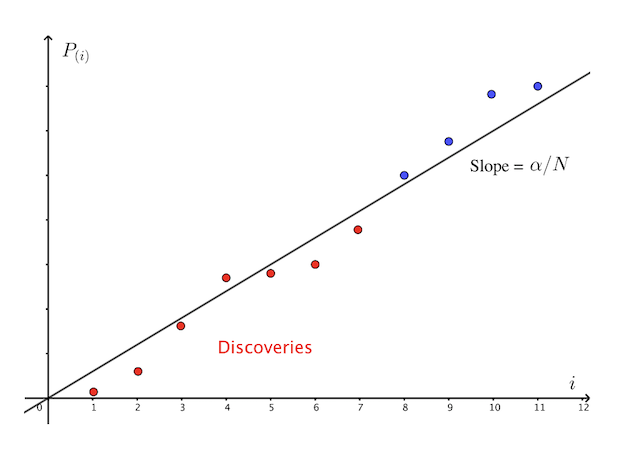
The BH procedure is as follows
- For each independent test, compute the p-value $p_{i}$. Sort the p-value from smallest to largest $p_{(1)} < \cdots < p_{(m)}$.
- Select \(R = \max\big\{i: p_{(i)} < \frac{i\alpha}{m}\big\}\).
- Reject null hypotheses with p-value $\leq p_{(R)}$.
By construction, this procedure rejects exactly $R$ hypotheses, and
\[p_{(R)} < \frac{R\alpha}{m} \Rightarrow \frac{p_{(R)}m}{R} < \alpha\]Let $m_{0} \leq m$ be the number true null hypotheses. Let $X_{i} = \mathbb{1}(p_{i} \leq p_{(R)})$ be whether hypothesis $i$ is rejected or not. Since $p_{i} \sim unif(0, 1)$, $X_{i} \sim bernoulli(p_{(R)})$. Under the assumption that tests are independent, $V = \sum_{i = 1}^{m_{0}}X_{i} \sim binomial(m_{0}, p_{(R)})$. Then by definition
\[FDR = \mathbb{E}\left(\frac{V}{R}\right) = \frac{1}{R}\mathbb{E}[V] = \frac{m_{0}p_{(R)}}{R} \leq \frac{mp_{(R)}}{R} < \alpha.\]In practice, the observed p-value $p_{i}$ is adjusted according to
\[p_{i}^{adj} = \min_{j = i, \dots ,m}\left(\min\left(\frac{m}{j}p_{(j)}, 1\right)\right)\]for $i = 1, \dots ,m$. The $i$-th null hypothesis is rejected if $p_{i}^{adj} \leq \alpha$. This results in exactly $R$ rejected null hypotheses because if $i \leq R$, then $p_{i}^{adj} < \alpha$, because
\[\begin{align*} p_{i}^{adj} = \min_{j = i, \dots ,m}\left(\min\left(\frac{m}{j}p_{(j)}, 1\right)\right) \leq \frac{m}{R}p_{(R)} < \alpha. \end{align*}\]The first inequality is from definition of minimum over a set that includes \(\frac{mp_{(R)}}{R}\), and the second inequality is by construction of \(\frac{m}{R}p_{(R)}\). If $i > R$, then $p_{i}^{adj} > \alpha$ because $p_{(R)}$ is defined as the last p-value in sorted p-values with $p_{(i)} < \frac{i\alpha}{m}$. Let us simulate 10 p-values from $unif(0, 0.3)$ and implement BH corrected p-values.
# simulation
n = 10
pvals = np.random.uniform(0, 0.3, size = n)

# implementation of benjamini-hochberg correction
def benjamini_hochberg(pvals):
    m = len(pvals)
    pAdj = [None] * m
    pvals.sort()
    pTransform = [m * pvals[i] / (i + 1) for i in range(m)]
    for i in range(m):
        minPTransform = min(pTransform[i:m])
        if minPTransform > 1:
            pAdj[i] = 1
        else:
            pAdj[i] = minPTransform
    return sorted([round(p, 7) for p in pAdj])

pAdj1 = benjamini_hochberg(pvals)
_, pAdj2, _, _ = multipletests(pvals, method = "fdr_bh", returnsorted = True)

print(pAdj1)
print(pAdj2)
[0.1788644, 0.1838926, 0.1940673, 0.1940673, 0.1940673, 0.1940673, 0.2294974, 0.2294974, 0.2294974, 0.2294974]
[0.17886437 0.18389261 0.19406731 0.19406731 0.19406731 0.19406731
 0.22949745 0.22949745 0.22949745 0.22949745]